examples.random_fields
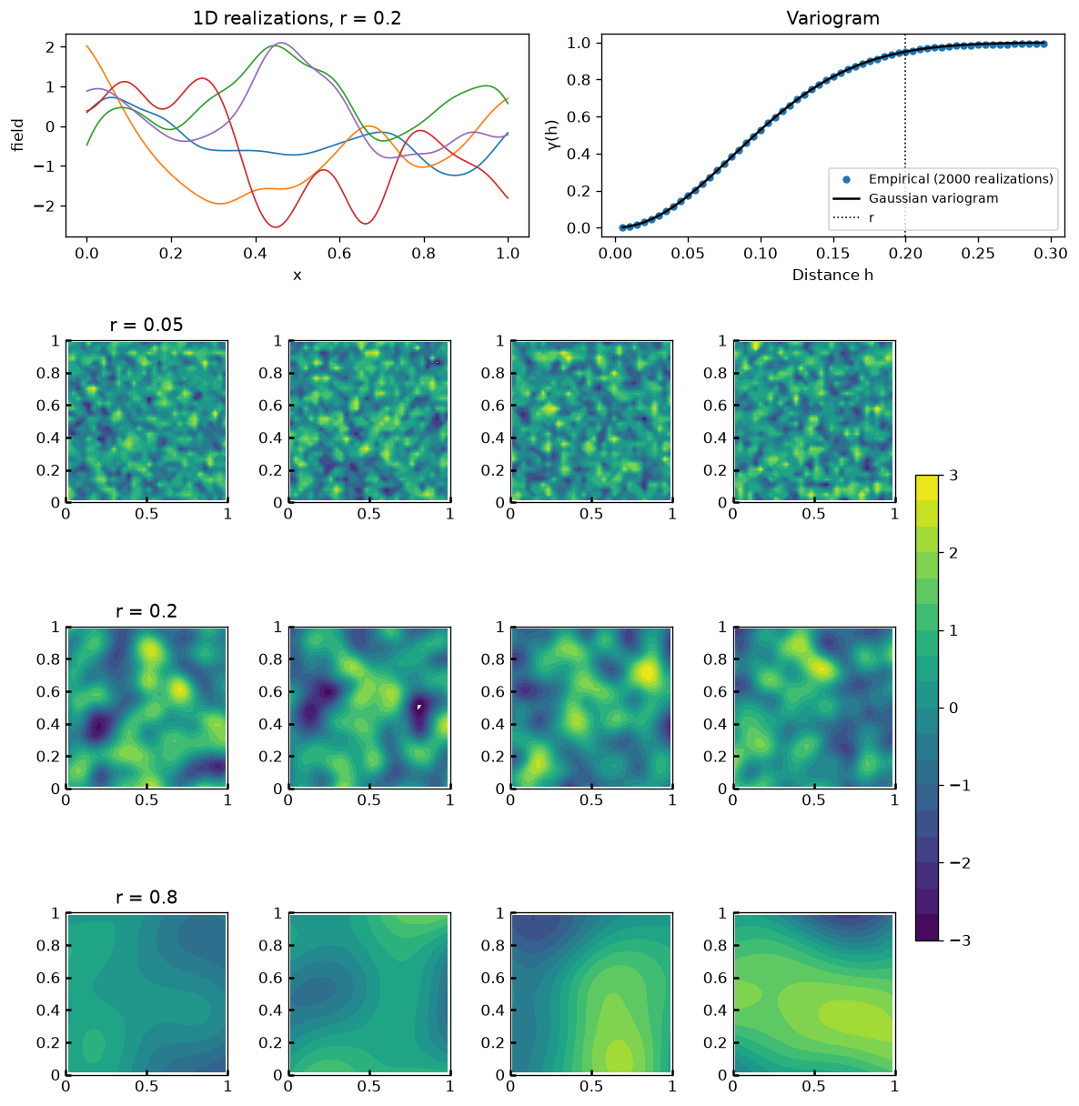
Gaussian random fields (minires.geostat), in 1D and 2D, and the effect of the range.
A permeability field to simulate on, or a prior to history match with, has to
come from somewhere. minires.geostat.gaussian_fields samples a stationary,
isotropic Gaussian field over the cell centres, from a Gaussian variogram
(minires.geostat.variogram_gauss) whose range, r, sets the length scale of
the heterogeneity. This is what the heterogeneous examples use for their
$ \log K $ (e.g. examples.water_cut_gradient), and what the tutorials of
HistoryMatching use for their
prior ensembles.
In the figure:
- Top left: a few realizations in 1D. Top right: their empirical variogram (half the mean squared difference between points a distance $ h $ apart, over many realizations) against the model's -- they agree, which is also asserted below: the sampler produces the covariance it claims to.
- Bottom: realizations in 2D, one row per range. A short range gives fine-grained heterogeneity, a long one smooth, large-scale trends -- with the same marginal distribution (standard normal) in every cell.
 1"""Gaussian random fields (`minires.geostat`), in 1D and 2D, and the effect of the range.
 2
 3A permeability field to simulate on, or a prior to history match with, has to
 4come from somewhere. `minires.geostat.gaussian_fields` samples a stationary,
 5isotropic Gaussian field over the cell centres, from a Gaussian variogram
 6(`minires.geostat.variogram_gauss`) whose range, `r`, sets the length scale of
 7the heterogeneity. This is what the heterogeneous examples use for their
 8$ \\log K $ (e.g. `examples.water_cut_gradient`), and what the tutorials of
 9[HistoryMatching](https://github.com/patnr/HistoryMatching) use for their
10prior ensembles.
11
12In the figure:
13
14- Top left: a few realizations in 1D. Top right: their *empirical* variogram
15  (half the mean squared difference between points a distance $ h $ apart,
16  over many realizations) against the model's -- they agree, which is also
17  asserted below: the sampler produces the covariance it claims to.
18- Bottom: realizations in 2D, one row per range. A short range gives
19  fine-grained heterogeneity, a long one smooth, large-scale trends -- with
20  the same marginal distribution (standard normal) in every cell.
21"""
22
23import matplotlib.pyplot as plt
24import numpy as np
25
26from minires import ResSim
27from minires.geostat import gaussian_fields, variogram_gauss
28from minires.plotting import show
29
30rng = np.random.default_rng(1)  # Reproducibility (the values are regression tested)
31
32## 1D: realizations, and the empirical variogram
33xx = np.linspace(0, 1, 201)
34r = .2
35fields_1d = gaussian_fields((xx,), N=2000, r=r, rng=rng)
36lags = np.arange(1, 60)
37h = lags * (xx[1] - xx[0])
38gamma_emp = np.array([np.mean((fields_1d[:, lag:] - fields_1d[:, :-lag])**2) / 2 for lag in lags])
39gamma_mod = variogram_gauss(h, r)
40assert np.allclose(gamma_emp, gamma_mod, atol=.05)
41
42## 2D: realizations for a few ranges
43model = ResSim(Lx=1, Ly=1, Nx=32, Ny=32)
44ranges = [.05, .2, .8]
45nShow = 4
46fields_2d = {r: gaussian_fields(model.mesh, N=nShow, r=r, rng=rng) for r in ranges}
47
48## Plot
49fig, axs = plt.subplots(num="Random fields", clear=True, nrows=1 + len(ranges), ncols=nShow,
50                        figsize=(10, 2.6 * (1 + len(ranges))))
51gs = axs[0, 0].get_gridspec()
52for ax in axs[0]:
53    ax.remove()
54ax = fig.add_subplot(gs[0, :2])
55ax.plot(xx, fields_1d[:5].T, lw=1)
56ax.set(title=f"1D realizations, r = {r}", xlabel="x", ylabel="field")
57ax = fig.add_subplot(gs[0, 2:])
58ax.plot(h, gamma_emp, "o", ms=4, label=f"Empirical ({len(fields_1d)} realizations)")
59ax.plot(h, gamma_mod, "k-", label="Gaussian variogram")
60ax.axvline(r, c="k", ls=":", lw=1, label="r")
61ax.set(title="Variogram", xlabel="Distance h", ylabel="γ(h)")
62ax.legend(loc="lower right", fontsize="small")
63kws: dict = dict(cmap="viridis", levels=np.linspace(-3, 3, 19), cticks=np.arange(-3, 4),
64                 wells=False, labels=False, finalize=False)
65for i, r in enumerate(ranges):
66    for j, ax in enumerate(axs[1 + i]):
67        h_ = model.plt_field(ax, fields_2d[r][j], colorbar=False,
68                             title=f"r = {r}" if j == 0 else None, **kws)
69fig.tight_layout()
70fig.colorbar(h_, ax=axs[1:].ravel().tolist(), ticks=kws["cticks"], shrink=.6, pad=.02)
71
72# Regression values, checked by `tests/test_examples.py`.
73__digest__ = dict(gamma_emp = gamma_emp,
74                  **{f"field_{i}": fields_2d[r][0] for i, r in enumerate(ranges)})  # per range
75
76if __name__ == "__main__":
77    show()