minires

MiniRes is a 2D, two-phase, black-oil, immiscible reservoir simulator using TPFA (two-point flux approximation).

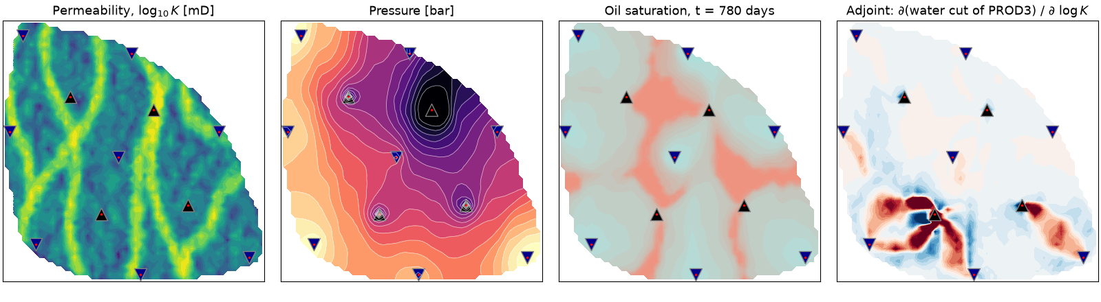
The Egg model: permeability, pressure, oil saturation, and the adjoint sensitivity of a producer's water cut

See examples for more demonstrations.

Governing equations

The simulator solves eqn. (1) and (2) (corresponding to (42) and (43) of the reference paper) :

$$\begin{align} - \nabla \cdot \mathbf{K} \lambda(s) \, \nabla p &= q \,, \tag{1} \cr \phi \frac{\partial s}{\partial t} + \nabla \cdot (f(s)\, \mathbf{v}) &= \frac{q_w}{\rho_w} \,. \tag{2} \end{align}$$

The quantities involved are all 2D-spatial fields, namely

$\phi \in [0, 1]$ is the porosity
$s \in [0, 1]$ is the water saturation
$p$ is the pressure
$v$ is the (volumetric) flow velocity ($\mathbf{v} = \mathbf{v}_o + \mathbf{v}_w$).
$q$ is the sources/sinks
$\rho$ is the density
$\mathbf{K}$ is the (absolute) permeability tensor: the rock's conductivity to flow, here diagonal, $\mathrm{diag}(K_x, K_y)$ per cell.
$\lambda(s)$ is the total mobility (sum of mobilities). Each (relative) mobility is the phase relative permeability divided by the phase viscosity, $\lambda_{\text{phase}} = k_{\text{phase}}/\mu_{\text{phase}}$.
- The relative permeabilities $k_{\text{phase}}(s) \in [0, 1]$ are a constitutive relation, not data: here, Corey (power-law) curves of the saturation rescaled by its residual values, with adjustable exponents and end-points, quadratic by default (ResSim.fluid, a minires.fluids.Fluid). Need not sum to 1.
- $\mu_{\text{phase}}$ is the phase viscosity, here constant.
$f(s) = \lambda_w(s) / \lambda(s) \in [0, 1]$ is the water fractional flow, giving $\mathbf{v}_w = f(s) \, \mathbf{v}$.

The right hand side of (2) is further simplified (relabelled) as $q$, i.e. dropping the $w$ (for "water") subscripts.

Derivation

Single phase

Conservation of mass in a porous ($\phi$) medium is expressed by

$$\frac{∂(\rho \phi)}{∂t} + ∇ \cdot (\rho \mathbf{v}) = q \,. \tag{3}$$

This equation is also called continuity eqn., advection eqn., transport eqn., or even 1st-order wave eqn. (if constant $v$). It says that divergence (or convergence) must be balanced by change in density or porosity, or sinks or sources. If we assume constant porosity, $\phi$, and incompressibility (constant $\rho$), then the time derivative vanishes, yielding the steady-state equation $$\nabla \cdot \mathbf{\mathbf{v}} = \frac{q}{\rho} \,. \tag{4}$$

We now have 1 equation and 2 unknowns (in 2D). Closing the system, Darcy's law provides 2 additional equations and 1 additional unknown, pressure $p$: $$\mathbf{v} = − \frac{\mathbf{K}}{\mu} \nabla u \,, \tag{5}$$ where $u = p - \rho g z \,.$ Analogously to Fourier's heat diffusion and Ohm's conduction law, Darcy's law (5) was initially derived empirically, but can be shown to be a special case of Navier-Stokes' momentum equation. It says that $\mathbf{v}$ is the gradient of the velocity potential, $u$, linearly transformed by the permeability tensor (matrix). Inserting the formula (5) into eqn. (4) yields $$− \nabla \cdot \frac{\mathbf{K}}{\mu} \nabla u = \frac{q}{\rho} \,. \tag{6}$$ which can be solved for $u$. In reservoir engineering, no-flow boundary conditions are most often used, and $u$ is only determined up to a constant (as behoves a potential). Finally, $u$ can be inserted in Darcy's law (5) to yield the (steady-state) velocity.

Two phases

Incompressibility again yields eqn. (4) for the total (volumetric) velocity.
Darcy's law (5) is assumed for each (both) individual phase, with $\mathbf{K}$ replaced by $\mathbf{K} \lambda_{\text{phase}}(s)$.
Neglecting $\nabla z$ (gravity, i.e. hydrostatic pressure), the flow potential, $u$, reduces to the pressure field, $p$.
Summing Darcy's law over the two phases yields $$\mathbf{v} = − \mathbf{K} \lambda (s) \nabla p \,. \tag{7}$$
Repeating the steps right above eqn. (6), one arrives at eqn. (1).
Meanwhile, immiscibility means that conservation of mass (3) must hold for each phase separately, i.e. the density $\rho$ gets replaced by $s_{\text{phase}} \, \rho_{\text{phase}}$, and $\mathbf{v}$ by $\mathbf{v}_{\text{phase}} = f_{\text{phase}}(s)\, \mathbf{v}$, immediately yielding eqn. (2).

How to solve

Equations (1) and (2) are nonlinearly coupled: $s$ and $p$ (yielding $v$ via eqn. (7)) appear in both equations. Trying to solve both equations simultaneously is a nonlinear root-finding problem, requiring Newton iterations and matrix inversions. In this context, it is tempting to use implicit time discretization (like ECLIPSE 100) where $s_{t+1}$ is expressed as a (nonlinear) function of itself, since this would also requires iterations

Here, instead, we apply sequential operator splitting, meaning that the two equations are solved independently, inserting the previous solution of (1) into (2), and vice-versa. Since it yields smaller systems (which can potentially be discretized explicitly) this is faster, but less accurate. When using an explicit (upwind) scheme for the nearly-hyperbolic saturation/transport equation, the strategy is called IMPES (implicit pressure, explicit saturation). The simulator also contains implicit saturation scheme, but it rarely outperforms the explicit one, ref ResSim.saturation_step_implicit.

The spatial discretization is carried out by finite volumes (FV), which is similar to finite differences (FD), but arguably easier to formulate for non-structured (irregular) grids (not our case). For the pressure equation, using only two points two approximate the transmissibility and fluxes at the interfaces is called it is called two-point flux approximation (TPFA); simple, but used widely (nearly default) in oil industry, due to its robustness and efficiency. Consider the equation $$- \nabla \cdot \lambda \nabla u = q \,, \tag{8}$$ where replacing $\lambda \leftarrow \mathbf{K} \lambda(s)$ reproduces eqn. (1), or $\lambda \leftarrow \mathbf{K}/\mu$ and $q \leftarrow q/\rho$ reproduces eqn. (6). FV methods apply the divergence theorem to eqn. (8) to replace point derivatives by integral quantities: interface fluxes and volumetric sources/sinks: $$- \int_{\partial \Omega_i} d x^2 \, \lambda \, (\nabla u) \cdot \mathbf{n} = \int_{\Omega_i} d x^3 \, q \,, \tag{9}$$ where $\Omega_i$ is the domain of cell index $i$, and $\partial \Omega_i$ is its boundary, with normal vector $\mathbf{n}$.

Now, in TPFA we approximate $(\nabla u) \cdot \mathbf{n}$ by a finite difference $$\delta u_{ij} := 2 \frac{u_j - u_i}{\Delta x_i + \Delta x_j}$$ where $u_i, u_i$ are the values of the potential, $u$, at centre of cells $i$ and $j$, which are located either side of the interface $\gamma_{ij}$, which is part of $\partial \Omega_i$. PS: by contrasts, mixed finite-element methods (FEM) do not approximate fluxes over cell edges but considers them unknown. Next, $\lambda$ is approximated by a harmonic average, $\lambda_{ij}$, including weights that account for the distances from the interface to the cell centres. Thus eqn. (9) becomes $$- \sum_j |\gamma_{ij}| \lambda_{ij} \delta u_{ij} = \int_{\Omega_i} d x^3 \, q \,, \tag{10}$$ where the sum is over the indexes $j$ of the interfaces around cell $i$. The left-hand side can be succinctly expressed as $- \sum_j t_{ij} (u_i - u_j)$, where $t_{ij}$ (see above their equation 17) is symmetric. Thus the whole linear system (for all $i$) is symmetric. Moreover, summing over $i$ yields $\sum_{ij} t_{ij} u_i - \sum_{ij} u_j = 0$, meaning that the vector of ones is a null vector for the system (as appropriate for a differential operator), and that $u$ is determined only up to an arbitrary constant (as appropriate for a potential). The constant is fixed, and the system is rendered invertible, by adding to the first element of the diagonal.

The system is thus symmetric positive definite, and is solved by conjugate gradients, preconditioned by a sparse LU factorization that is cached across the time steps (ResSim.cached_precond).

The pressure system need not be factorized afresh each step.

Its matrix changes only through the mobility $λ(s)$, so the factorization of an earlier step is an excellent preconditioner for the current one, at the cost of a back-substitution, and a refactorization only once the iteration stalls. tests/test_precond.py benchmarks.

Units

The units are by default SI (m, s, Pa). But you can switch to metric (m, day, bar, mD) or field-like (ft, day, psi) by changing ResSim.cdarcy.

Compressibility

The above is the default incompressible model, which is what the reference paper treats. Below we derive the so-called slightly compressible approximation, switched on by setting minires.ResSim.ct ($c_t$) $> 0$.

Definition

The compressibility of anything (rock or fluid) is the relative change of its volume by pressure, $c = -\frac{1}{V} \frac{\partial V}{\partial p}$. For rock (pores) it becomes $c_r = \frac{1}{\phi} \frac{\partial \phi}{\partial p}$, while for fluids it is $c_f = \frac{1}{\rho} \frac{\partial \rho}{\partial p}$. With two phases, the fluid in the pores is a mixture, so that the total compressibility is the saturation-weighted sum $c_t = c_r + s_w c_w + s_o c_o$.

Approximation

The model, however, holds it as a single constant, ct, so it is accurate to $O(c_t)$ alone -- the slightly of slightly compressible, which is reasonable for liquids, but not for gas. Thus $\rho \propto e^{c (p - p_0)}$, which the approximation retains only to first order, $\rho \approx \rho_0 [1 + c (p - p_0)]$: a density affine in $p$.

Note that $\rho(p)$ (and thus nonlinearity in $p$) also appears through the source term (wells): a rate fixed at the surface moves a reservoir volume $\propto 1/\rho(p)$. Here it is approximated as a constant (the formation volume factor $B = 1$), or, for a BHP well, as linear in $p$ (Peaceman).

Derivation

Return to the conservation of mass (3), now with $\rho = \rho(p)$ and $\phi = \phi(p)$. By the chain rule and the definitions (constant $c$) above, the accumulation term becomes $$\frac{\partial (\rho \phi)}{\partial t} = \rho \, \phi \, (c_r + c_f) \, \frac{\partial p}{\partial t} \,,$$ where $c_f$ is the compressibility of the fluid filling the pores. Meanwhile, in the flux term, $\nabla \cdot (\rho \mathbf{v}) = \rho \, \nabla \cdot \mathbf{v} + \mathbf{v} \cdot \nabla \rho$, the latter term is $O(c)$ relative to the former (since $\nabla \rho = \rho \, c \, \nabla p$ thanks to constant $c$), and is therefore dropped, an approximation equivalent to the affine one above. Dividing by $\rho$ and inserting Darcy's law (7), we recover eqn. (1) except now with a time derivative: $$\phi \, c_t \frac{\partial p}{\partial t} - \nabla \cdot \mathbf{K} \lambda(s) \, \nabla p = q \,. \tag{11}$$ Eqn. (11) is parabolic: a diffusion equation for pressure, whose coefficient $\eta = \mathbf{K} \lambda / (\phi \, c_t)$ is the (pressure, or hydraulic) diffusivity.

The transport equation (2) needs a corresponding term. The total velocity is no longer divergence-free: by eqn. (11) and reverting Darcy's law (7), $\nabla \cdot \mathbf{v} = q - \phi \, c_t \, \partial p / \partial t$, so the storage must be charged to the phases. This model does so in proportion to their saturation, $$\phi \frac{\partial s}{\partial t} + s \, \phi \, c_t \frac{\partial p}{\partial t} + \nabla \cdot (f(s)\, \mathbf{v}) = q_w \,, \tag{12}$$ which is what makes the water and oil equations sum to eqn. (11), so that e.g. depleting a fully water-saturated reservoir leaves $s = 1$, rather than conjuring oil out of the produced volume. (Deriving each phase equation individually would instead charge the water $s \, (c_r + c_w) \, \phi \, \partial p / \partial t$; the two coincide iff $c_w = c_o$, the difference being within the $O(c_t)$ fidelity anyway.) Ref minires.ResSim.storage_rate. Both new terms vanish for $c_t = 0$, recovering eqns. (1) and (2) exactly.

Consequences

The now parabolic pressure equation (11) is discretized here by backward Euler over the same $\Delta t$ as the saturation step, which adds $\phi \, c_t \, h^2 / \Delta t$ to the diagonal of the system (10), rendering it nonsingular without pinning. Thus the solution method survives. The sequential splitting remains applicable, and the pressure step is still one sparse linear solve, with no Newton iteration on $p$, and no PVT properties ($\rho$, $\mu$, $B$, $\phi$) to update with the pressure.

The absolute pressure level is meaningful, so an initial pressure must be given. However, the datum remains arbitrary. Eqn. (11) involves $p$ only through its derivatives, so shifting P0 (and any BHP targets) by a constant shifts the whole pressure trajectory by it, leaving saturations and rates untouched. The level is thus consequential (unlike for $c_t = 0$, it is propagated, not free) but only relative to the initial one. An absolute pressure would enter only through pressure-dependent properties -- precisely what the approximation drops.
Sources and sinks need not balance. The imbalance -- the voidage, production minus injection -- is supplied by expansion, permitting primary depletion by a lone producer. Summing the rows of the system (ref tests/test_compressible.py) yields $c_t \, \Delta \bar{p} = V_{\text{voidage}} / V_{\text{pore}}$, so the fidelity requirement, $c_t \, \Delta p \ll 1$, is a matter of the voidage asked of the fluids, not of choosing ct small. Linearity again: the mean pressure declines in proportion to the cumulative voidage, whatever its distribution in space or time -- the straight line of the material-balance plot (ref "Vocabulary"), by which pore volume is estimated.
Pressure is transient rather than instantaneous: $\sqrt{\eta t}$ is the radius of investigation, how far a well has "felt" after time $t$. Flow is called transient while that radius is still growing, and pseudo-steady state (or boundary-dominated) once it has reached the whole of the drainage volume, whereafter the pressure declines uniformly. Well testing is the inverse problem of inferring $\mathbf{K}$ and the skin (ref minires.wells.peaceman_WI) from a measured transient, typically during the build-up after shutting a well in -- as examples.buildup does. By the linear approximations, superposition holds, in space and in time: a shut-in is a flowing well plus an equal and opposite one started at the shut-in, and the pressure anywhere is the sum of the wells' individual transients. This is what makes well testing an analytical inference method -- the line-source solution, the Horner plot, and the semilog-derivative plateau that examples.buildup reads $\mathbf{K}$ off, are all solutions of the linear diffusion equation.

Vocabulary of reservoir engineering

Reservoir simulators implement porous media flow on upscaled geophysical parameters typically with grid blocks between 1 - 100 m. They usually parameterize multiphase flow. If only the two phases of oil and water are used it is called black-oil. A common assumption is that the flow is immiscible: not mixing (oil and water). But this does not mean that gas cannot be dissolved in oil.

Fossil fuel hydrocarbons is sedimented, pressurized, organic material (mostly plants?) that used to live on the sub-sea continental shelves On-land organic material turns into coal. ⇒ Saudi-Arabia used to be sub-sea? The energy in oil & gas comes from the sun (photosynthesis), not the compression.

The lightest hydrocarbons (methane, ethane, etc.) usually escapes quickly, while oils moves slowly towards the surface. Sometimes the geology is bends to form caps of non-permeable rock, so that the migrating hydrocarbons are trapped. Upon drilling, unless valves are in place, the pressure of the initial equilibrium will cause a blow out. A new equilibrium is usually attained when 20% of the hydrocarbons have been produced, which marks the end of the primary production. In the North Sea, these reservoirs lie 1000-3000 meters below the sea bed. Norway is also surrounded by the Norwegian sea, and the Barents sea, towards Murmansk.

Porosity, $\phi$, is the void volume fraction. Depends on pressure, because rock is compressible. Compressibility is the porosity's (relative) gradient wrt. pressure. Usually neglected, so that $\phi$ is a constant, but spatial, field.

Permeability, denoted by tensor $\mathbf{K}$, quantifies transmissibility. Usually SPD, and correlated with $\phi$. Among the reservoir rocks, sandstone usually have large, well-connected pores, and high permeability, shale is nearly impermeable, like cap rock and bed rock. Permeability is measured in Darcy ($≈ 10^{-12} m^2$). A medium is called isotropic if $\mathbf{K}$ is scalar.

The phases (rock, oil, gas), whose saturations sum to $1$, contains components (e.g. methane, ethane, propane), usually grouped as pseudo-components. Each phase's mass fraction component, $c_{phase,i}$, sums to $1$. Each phase has density, $\rho$ and viscosity, $\mu$, generally functions of the phase pressure, but usually neglected except for gas. The differences in pressure are named capillary pressure because they arise due to interfacial tensions. A phase's compressibility is defined similar as for the rock's. Confusingly, it is also denoted with $c$, but using only a single subscript.

Phases do not really mix. But in macro-scale modelling all phases may be present at the same location. Therefore a phase's permeability should depend on the saturations, to which end we introduce relative permeability, $k_{r,i} = k_{r,i}(s_g, s_o), i = g, o, w$ a nonlinear function, yielding an (effective) permeability $\mathbf{K_i} = \mathbf{K} k_{r,i}$ Relative permeability curves do not extend all over the interval $[0, 1]$. The smallest saturation where a phase is mobile is called the residual saturation. This adsorption effects may vary, and this may have important effects, particularly for simulation of polymer injection. The uncertainty regarding relative permeability is modest compared to the enormous uncertainty of the rock permeability.

Everything depends on thermodynamics, but this is often complex and neglected, except perhaps for the bubble/boiling point pressures, which govern how much of the gas dissolves in oil.

Since compressibility relates volumes to pressure, a volume must be qualified by where it is measured. The formation volume factor, $B$, is the ratio of the volume at reservoir conditions to that of the same mass at the surface ("stock tank"), and is how field rates (measured at the surface) are converted to the reservoir rates that a simulator works in. This model has $B = 1$. Related PVT (pressure-volume-temperature) vocabulary: the bubble point is the pressure below which gas comes out of solution; an oil above it is undersaturated, and the amount of gas it holds is the solution gas-oil ratio, $R_s$.

The drive mechanism is whatever supplies the energy that pushes the hydrocarbons to the well. Fluid and rock expansion (a.k.a. depletion drive), which is what $c_t > 0$ enables here in the absence of injection, is the weakest, recovering only a few percent, because $c_t$ is so small. Stronger ones are solution gas drive, gas cap drive, water drive (aquifers), gravity drainage, and compaction drive (which manifests as seabed subsidence). Recovery is staged: primary production runs on the native drive; secondary adds pressure support by injecting water or gas (waterflooding being the case simulated here); tertiary, or EOR (enhanced oil recovery), alters the flow physics itself, e.g. by polymer, surfactant, or CO₂ injection. The voidage replacement ratio is the injected reservoir volume divided by the produced one; $\mathrm{VRR} = 1$ is exactly the balance, $\sum q = 0$, that the incompressible model is obliged to impose. The zero-dimensional (single tank) accounting of all of the above, used to estimate reserves without a grid, is called material balance.

Aquifers are beneficial in reservoirs as they act as pressure compensators. Oil production ⇒ pressure decrease ⇒ aquifers expansion ⇒ pressure compensation. Despite consisting of water, the expansion is generally significant because the base volume is so big, or the aquifer might even be connected to the ocean.

Other lingo: water table, facies, channels, fissures, fractures.

View Source

 1""".. include:: README.md"""
 2
 3from minires.core import ResSim
 4from minires.grid import Fluxes, Grid2D
 5from minires.fluids import Fluid
 6from minires.wells import Wells, aquifer_WI, peaceman_WI, well_path
 7
 8# Also pdoc's table of contents: `ResSim` is documented on the package page (beside the
 9# README), and the listed submodules on their own pages. `core` is deliberately absent,
10# lest `ResSim` be documented twice; so are the other re-exports, which are documented
11# in their home modules.
12__all__ = ["ResSim", "grid", "wells", "fluids", "plotting", "tlm"]

@dataclass

class ResSim(minires._repr.AlignedRepr, minires.grid.Grid2D, minires.plotting.Plot2D): View Source

 20@dataclass
 21class ResSim(AlignedRepr, Grid2D, Plot2D):
 22    """Reservoir simulator class.
 23
 24    Implemented with OOP (instead of passing around dicts) to facilitate
 25    bookkeeping of ensemble forecasting
 26    (where parameter values of one instance should not influence another)
 27
 28    Example:
 29    >>> model = ResSim(Lx=1, Ly=1, Nx=64, Ny=64, wells=[
 30    ...     dict(xy=[0, .32], rate=+1),   # injector
 31    ...     dict(xy=[1, 1], rate=-1),     # producer
 32    ... ])
 33    >>> water_sat0 = np.zeros(model.Nxy)
 34    >>> dt = .35
 35    >>> nSteps = 2
 36    >>> S, P = model.sim(dt, nSteps, water_sat0, pbar=False)
 37
 38    This produces the following values (used for automatic testing):
 39    >>> S[-1, [100, 1300, 2900]]
 40    array([0.9429345 , 0.91358172, 0.71554613])
 41    """
 42
 43    # Dont use dataclass repr
 44    __repr__ = AlignedRepr.__repr__
 45
 46    # Prefer __setattr__ approach (over @property get/set-ers)
 47    # because @property requires the _private pattern,
 48    # which is pretty ugly with dataclasses.
 49    def __setattr__(self, key: str, val: Any) -> None:
 50        # Defaults that the dataclass cannot express, depending as they do on the grid
 51        if val is None:
 52            if key == "K":
 53                val = np.ones((2, *self.shape))
 54            elif key == "por":
 55                val = np.ones(self.shape)
 56            elif key == "active":
 57                val = np.ones(self.shape, bool)
 58        # Permeabilities
 59        if key == "K" and val is not None:
 60            if np.isscalar(val):
 61                val = np.full(self.shape, val, dtype=float)
 62            if val.size == self.size:
 63                val = np.stack([val, val])  # both components
 64            val = val.reshape((2, *self.shape))
 65        # Active cells: the first is where `TPFA` pins the incompressible pressure
 66        if key == "active" and val is not None:
 67            val = np.asarray(val, bool).reshape(self.shape)
 68            assert val.any(), "No active cells."
 69            self._pin = int(np.argmax(val))
 70        # Fluid: a dict (or `None`) builds the `Fluid` it parameterizes
 71        if key == "fluid":
 72            if val is None:
 73                val = Fluid()
 74            elif isinstance(val, dict):
 75                val = Fluid(**val)
 76        # Wells -- records (or `None`) get assembled into a `Wells`, which then
 77        # gets bound, whereupon it snaps its completions onto this grid.
 78        # NB: the wells' own normalization is `minires.wells.Wells.__setattr__`.
 79        if key == "wells":
 80            if not isinstance(val, Wells):
 81                val = Wells.from_records(self, val)
 82            val._bind(self)
 83        # Set
 84        super().__setattr__(key, val)
 85
 86    def __getstate__(self) -> dict:
 87        # The cached factorization (ref `cached_precond`) is a `SuperLU`, which
 88        # cannot be pickled -- and is a mere cache, so `deepcopy` and
 89        # multiprocessing (as HistoryMatching does) simply leave it behind.
 90        state = self.__dict__.copy()
 91        state.pop("_pLU", None)
 92        return state
 93
 94    name: str = "Unnamed"
 95    """Description."""
 96
 97    cdarcy: float = 1.0
 98    """Unit conversion factor for Darcy's law, $C$ -- ECLIPSE's `CDARCY`.
 99
100    If you want to change unit system you not only need to manually convert
101    the dimensional input quantities to the new units, but also change $C$ according to
102    $$ C = \\frac{u_k \\, u_p \\, u_t}{u_μ \\, u_L^2} \\,, $$
103    (with $u_k$ the SI magnitude of the unit chosen for $k$).
104    Any *coherent* system gives `1`: choose base units for length, time and mass,
105    derive $u_p = M/(L T^2)$, $u_μ = M/(L T)$ and $u_k = L^2$ from them.
106
107    | System | $u_L$ | $u_t$ | $u_p$ | $u_k$ | $u_μ$ | rate | $C$ |
108    |---|---|---|---|---|---|---|---|
109    | SI | m | s | Pa | m² | Pa·s | m²/s | `1` |
110    | CGS | cm | s | barye | cm² | poise | cm²/s | `1` |
111    | MTS | m | s | pièze | m² | pz·s | m²/s | `1` |
112    | mm-ms-g | mm | ms | MPa | mm² | kPa·s | mm²/ms | `1` |
113    | Darcy's own | cm | s | atm | darcy | cP | cm²/s | `1` |
114    | metric | m | day | bar | mD | cP | m²/day | `0.008527` |
115    | field-like | ft | day | psi | mD | cP | ft²/day | `0.006328` |
116    | lab | cm | hour | atm | mD | cP | cm²/hour | `3.6` |
117
118    .. note:: The rate unit is forced to $u_L^2/u_t$ -- an areal rate.
119
120        A well rate of `20` for a 25 m thick reservoir means 500 m³/day.
121
122    .. note:: $C$ enters at exactly 2 sites, both of them Darcy's law.
123
124        The transmissibilities of `TPFA` and the well index of
125        `minires.wells.peaceman_WI`. Everything else is derivative, and
126        already consistent.
127    """
128
129    fluid: Any = None
130    """The two-phase fluid: a `minires.fluids.Fluid`, holding the viscosities
131    and the Corey relative permeability parameters, and computing the mobilities
132    and fractional flow from them.
133
134    Assigning a `dict` builds one (`ResSim(fluid=dict(vo=5, swc=.2))`), and `None`
135    the default (unit viscosities, the reference paper's quadratic curves). Its
136    fields stay writable (`model.fluid.vo = 5`). A `Fluid` subclass (e.g. with
137    tabulated curves) may be assigned instead.
138    """
139    ct: float = 0.0
140    """Total (rock + fluids) compressibility, $c_t$, as a single constant.
141
142    The default, `0`, yields the incompressible model, whose pressure eqn. is
143    elliptic: pressure is defined only up to an additive constant, and the
144    sources/sinks must balance. Setting `ct > 0` yields the *slightly
145    compressible* model: the pressure eqn. gains the accumulation term
146    $ φ \\, c_t \\, ∂p/∂t $ (discretized by backward Euler over the same `dt` as
147    the saturation step, which is what makes `P0` of `sim` consequential), and
148    the transport eqn. the matching storage term, charged to the phases in
149    proportion to their saturation (ref `storage_rate`). Injection and
150    production then need not balance, enabling e.g. primary depletion.
151
152    Derivation, fidelity ($ c_t \\, Δp \\ll 1 $, which the voidage sets, not
153    `ct`) and vocabulary: ref the "Compressibility" section of the docs.
154    """
155    cached_precond: bool = True
156    """Solve the pressure system iteratively, preconditioned by a cached factorization.
157
158    The alternative (`False`) is a fresh sparse direct factorization each
159    time step. But the system changes slowly -- only through the mobility
160    $λ(s)$, i.e. where the front has moved -- so the factorization of an
161    *earlier* step remains an excellent preconditioner: with it, conjugate
162    gradients converges in 1--2 iterations if the saturation is (nearly)
163    static, and in ~12 behind a moving front (each the cost of one
164    back-substitution, i.e. 1/30 of a factorization). The factorization is
165    refreshed only when convergence fails (as it does when the mobility has
166    drifted too far, e.g. after many steps at a strong viscosity contrast),
167    so the result is exact to the solver tolerance (`1e-10`) either way. It
168    requires the system to be SPD, which the TPFA system is (ref the "How to
169    solve" section of the docs).
170
171    The cache is per instance (`_pLU`) and is dropped on pickling and
172    `deepcopy`, a `SuperLU` not being picklable; a copy simply refactorizes
173    on its next step. The measurements (2--6x on the well-test and depletion
174    examples, 15--40% on the waterfloods), and what was tried besides, are
175    recorded in `tests/test_precond.py`.
176    """
177
178    # NB: the array attributes are typed `Any` since `__setattr__` normalizes
179    # whatever array-like (nested lists, scalars) is assigned to them.
180    K: Any = None
181    """Permeabilities (in x and y directions). Array of shape `(2, Nx, Ny)`)."""
182    por: Any = None
183    """Porosity; Array of shape `(Nx, Ny)`)."""
184    active: Any = None
185    """Mask of the active cells, `(Nx, Ny)`, boolean. Default: all `True`.
186
187    Setting some cells inactive carves an irregular reservoir out of the
188    rectangular grid -- an outline, holes, or a (sealing) fault: a line of
189    inactive cells, which blocks flow so long as it is unbroken (a diagonal
190    staircase suffices, fluxes passing only through faces). Inactive cells
191    take no part in the physics:
192
193    - The faces to them carry zero transmissibility, hence zero flux, so the
194      reservoir is closed along their perimeter as it is along the boundary.
195    - They have no equations. The pressure system carries an identity row for
196      each (keeping it well conditioned, unlike a tiny permeability would), and
197      their pore volume is taken as infinite (ref `pore_volume`; so they never
198      bind the CFL, as a tiny porosity would). So their state is simply carried
199      through `sim` unchanged from `S0` and `P0`. Plots mask them out.
200    - A well may not be completed in one (`_validate` checks). Should the
201      active cells form several disconnected regions, each is a reservoir of
202      its own, and only the first is pinned (ref `TPFA`): if `ct == 0`, the
203      others must balance their own rates, or hold a BHP well -- which is not
204      checked as such, but the singular system it would otherwise make is
205      caught by the residual check of `_solve_pressure`.
206
207    The arrays (`K`, `por`, `S0`, ...) keep the full grid shape, and the flat
208    index (`xy2ind`) runs over all cells: the mask selects the active ones.
209    """
210
211    wells: Any = None
212    """The wells: a `Wells`, holding the flat, per-*completion* arrays --
213    positions, rates, pressures, well indices -- that the model runs on.
214
215    Assigning a list (or `dict`) of records -- one per well -- assembles one,
216    which is the convenient way to configure them; the record format is
217    documented in `minires.wells.Wells.from_records`. Assigning `None`
218    empties it. A `Wells` may also be given directly, in which case it is
219    *bound* to this model, whereupon its completions snap onto the grid.
220
221    The arrays remain writable throughout (`model.wells.rates = ...`), as an
222    ensemble or optimisation loop requires.
223    """
224
225    def pore_volume(self) -> np.ndarray:
226        """Pore volume (per unit thickness) of each cell, `h2 * por`. Flat.
227
228        `inf` for inactive cells (ref `active`): dividing by it, the transport
229        schemes leave their saturation alone, and the CFL estimate ignores them.
230        """
231        pv = self.h2 * self.por.ravel()
232        return np.where(self.active.ravel(), pv, np.inf)
233
234    nComp = property(lambda self: self.wells.nComp)
235    """Num. of well *completions*, i.e. the rows of every array the model
236    indexes by them -- which is what it actually solves for, the equations
237    being assembled per completion.
238    Forwarded from `minires.wells.Wells.nComp`.
239    """
240
241    def assemble_wells(
242        self, S: np.ndarray | None, P: np.ndarray | None, k: int
243    ) -> None:
244        """Set up (for time `k`) the wells' contributions to the equations.
245
246        The controls are those of `well_controls`, to which `S` and `P` (the
247        state at the *start* of the step) are simply passed on.
248        Rate-controlled wells enter the source/sink *field*, `_Q`, directly.
249        BHP-controlled ones (ref `minires.wells.Wells.bhp`) cannot: their
250        rate is not yet known. They instead enter the pressure equations in
251        `TPFA`, after which `realize_bhp` folds the resulting rate into `_Q`.
252        """
253        ctrl = self.well_controls(S, P, k)
254        inds = self.xy2ind(*self.wells.xy.T)
255        rates, p_bh = ctrl["rates"], ctrl["bhp"]
256        is_bhp = np.isfinite(p_bh)
257        assert np.isfinite(rates[~is_bhp]).all(), (
258            "A rate-controlled well has a non-finite rate. Give it a number"
259            " (`0` shuts it in), or put it on BHP control; ref `Wells.rates`."
260        )
261
262        # The well model's constant of proportionality, WI * λ_t.
263        # NB: `nan` marks the rate-controlled wells, throughout.
264        WI_lam = np.full(self.nComp, np.nan)
265        if is_bhp.any():
266            WI = self.wells.WI
267            assert WI is not None and np.isfinite(WI[is_bhp]).all(), (
268                "BHP control requires (finite) `Wells.WI`."
269            )
270            assert S is not None, "BHP control requires `S` (for λ_t)."
271            Mw, Mo = self.fluid.RelPerm(S)
272            WI_lam[is_bhp] = WI[is_bhp] * (Mw + Mo)[inds[is_bhp]]
273
274        # Translate well conditions for cells.
275        # NB: Dont use `Q[inds] += ...` since `inds` may contain dupes.
276        self._Q, bhp_diag, bhp_rhs = np.zeros((3, self.Nxy))
277        np.add.at(self._Q, inds[~is_bhp], rates[~is_bhp])
278        np.add.at(bhp_diag, inds[is_bhp], WI_lam[is_bhp])
279        np.add.at(bhp_rhs, inds[is_bhp], (WI_lam * p_bh)[is_bhp])
280        rates[is_bhp] = np.nan  # only `realize_bhp` knows these
281        self._wells_now: dict[str, np.ndarray] = dict(
282            inds=inds, rates=rates, p_bh=p_bh,
283            WI_lam=WI_lam, bhp_diag=bhp_diag, bhp_rhs=bhp_rhs,
284        )  # fmt: skip
285
286    def realize_bhp(self, P: np.ndarray) -> None:
287        """Compute rates for BHP wells. Enter into `_Q` and `_wells_now["rates"]`.
288
289        The rate, $ WI λ_t (p_\\mathrm{bh} - p_\\mathrm{cell}) $, is signed by
290        nature (ref the `minires.wells.Wells.bhp` warning).
291
292        By construction of the linear system of `TPFA`, this leaves `_Q` equal
293        to the *total* well flux, which is what keeps `storage_rate` -- and
294        hence the transport step -- consistent with the pressure solution.
295        """
296        wls = self._wells_now
297        WI_lam = wls["WI_lam"]  # `nan` marks the rate-controlled wells
298        # Insert in cell source/sink field
299        self._Q = self._Q + wls["bhp_rhs"] - wls["bhp_diag"] * P
300        # Insert in per-well rates
301        is_bhp = np.isfinite(WI_lam)
302        wls["rates"][is_bhp] = (WI_lam * (wls["p_bh"] - P[wls["inds"]]))[is_bhp]
303
304    def _record_actual_well_operation(
305        self, S: np.ndarray, P: np.ndarray, k: int
306    ) -> None:
307        """Record `actual_rates`/`actual_bhp`. Warn about flow direction flip."""
308        wls = self._wells_now
309        if k:
310            is_bhp = np.isfinite(wls["WI_lam"])
311            flipped = is_bhp & (wls["rates"] * self.wells.actual_rates[:, k - 1] < 0)
312            if flipped.any():
313                warnings.warn(
314                    f"BHP-controlled well(s) {np.flatnonzero(flipped).tolist()}"
315                    f" reversed flow direction at step {k}"
316                    " (an inflow injects water); ref `Wells.bhp`.",
317                    stacklevel=2,
318                )
319        self.wells.actual_rates[:, k] = wls["rates"]
320        self.wells.actual_bhp[:, k] = self.bhp(S, P, wls["rates"])
321
322    def well_controls(self, S: np.ndarray | None, P: np.ndarray | None, k: int) -> dict:
323        """Compute the wells' controls for time `k`: `dict(rates=..., bhp=...)`.
324
325        Each is a `(nComp,)` array, read off the specifications --
326        `minires.wells.Wells.rates`, `minires.wells.Wells.bhp` -- which
327        are *open-loop*: fixed before the simulation begins. Overriding
328        (patching/subclassing) this method is therefore how to do *feedback*
329        control, the controls being free to depend on the state at the *start*
330        of the step: the saturation `S` and the pressure `P`.
331        The returned arrays are copies, so they may be modified in place.
332
333        Most feedback concerns the rates alone -- e.g. shutting the wells upon
334        water breakthrough at the producer:
335
336        >>> class Shutter(ResSim):
337        ...     def well_controls(self, S, P, k):
338        ...         ctrl = super().well_controls(S, P, k)
339        ...         if S is not None and S[self.xy2ind(1, 1)] > .5:
340        ...             ctrl["rates"][:] = 0    # NB: all of them! See warning
341        ...         return ctrl
342        >>> model = Shutter(Lx=1, Ly=1, Nx=16, Ny=16,
343        ...                 wells=Wells(xy=[[0, 0], [1, 1]], rates=[[1], [-1]]))
344        >>> SS, PP = model.sim(.05, 20, model.fluid.swc*np.ones(model.Nxy), pbar=False)
345        >>> int((model.wells.actual_rates[1] == 0).argmax())  # step of breakthrough
346        16
347
348        But the `bhp` is here too, and with it each well's *control mode*
349        (`nan` => rate-controlled, ref `minires.wells.Wells.bhp`) -- which
350        is what an approximate mode *switch* requires. For example, rate
351        control with a BHP limit -- the industrial default -- wherein a
352        producer holds its rate only for as long as that does not draw it
353        below some `p_min`:
354
355        >>> class Limited(ResSim):
356        ...     p_min = .5
357        ...     def well_controls(self, S, P, k):
358        ...         ctrl = super().well_controls(S, P, k)
359        ...         if P is None:
360        ...             return ctrl                    # nothing to switch on
361        ...         p_bh = self.bhp(S, P, ctrl["rates"])
362        ...         switch = p_bh < self.p_min         # the rate is unsustainable
363        ...         ctrl["bhp"] = np.where(switch, self.p_min, np.nan)
364        ...         return ctrl
365        >>> model = Limited(Lx=1, Ly=1, Nx=16, Ny=16, ct=.1,
366        ...                 wells=Wells(xy=[[.5, .5]], rates=[[-.25]]))
367        >>> from minires import peaceman_WI
368        >>> model.wells.WI = peaceman_WI(model, model.wells.xy, rw=1e-3)
369        >>> SS, PP = model.sim(.02, 25, np.zeros(model.Nxy),
370        ...                    P0=np.ones(model.Nxy), pbar=False)
371
372        The well delivers its target rate until the limit binds, and declines
373        thereafter -- at constant $ p_\\mathrm{bh} $, exponentially so
374        (ref `examples/well_control.py`, which plots all three modes):
375
376        >>> (-model.wells.actual_rates[0, [0, 5, 6, -1]]).round(3)
377        array([0.25 , 0.25 , 0.182, 0.005])
378
379        .. warning:: With `ct == 0` the rates must still sum to 0 at every step.
380
381            Ref `minires.wells.Wells.rates`. So shutting one well requires
382            matching it on the other side -- as above.
383
384        .. note:: The mode switch lags the solve by one step.
385
386            It is decided from the previous step's pressure, whereas the well
387            model itself is solved *simultaneously* with the new one. So the
388            limit is breached for the one step in which it comes to bind.
389            Shorten `dt` to refine.
390
391        .. note:: `S` and `P` may be `None`, so an override should tolerate that.
392
393            They are `None` if the caller has none to offer -- as when
394            `assemble_wells` is used merely to set up a plot.
395
396        .. note:: Setting both controls for a well is not an error, just pointless.
397
398            `assemble_wells` discards the rate of a BHP-controlled well -- it
399            is `realize_bhp` that fills it in.
400        """
401        return dict(
402            rates=self.wells.at_time("rates", 0.0, k),
403            bhp=self.wells.at_time("bhp", np.nan, k),
404        )
405
406    def bhp(self, S: np.ndarray, P: np.ndarray, rates: np.ndarray) -> np.ndarray:
407        """Bottom-hole pressures implied by the (signed) `rates`, via the well indices.
408
409        I.e. the well model of `minires.wells.Wells.WI`, solved for
410        $ p_\\mathrm{bh} $:
411        the rate's sign puts an injector above, a producer below, its cell
412        pressure. `nan` wherever the well index is unset.
413
414        `S` and `P` (both flat) should be the saturation and the pressure of the
415        *same* `pressure_step`, i.e. `SS[k]` and `PP[k+1]` of `sim` -- which is
416        what `actual_bhp` records, so prefer reading that.
417
418        .. warning:: $ λ_t $ is that of the well's *cell*.
419
420            So an injector's injectivity is governed by the mobility of
421            whatever the cell currently holds, rather than by that of the
422            injectant.
423        """
424        if self.wells.WI is None:
425            return np.full(self.nComp, np.nan)
426        Mw, Mo = self.fluid.RelPerm(S)
427        ii = self.xy2ind(*self.wells.xy.T)
428        return P[ii] + rates / (self.wells.WI * (Mw + Mo)[ii])
429
430    # Pres() -- listing 5
431    def pressure_step(
432        self,
433        S: np.ndarray,
434        P: np.ndarray | None = None,
435        dt: float | None = None,
436    ) -> tuple[np.ndarray, Fluxes]:
437        """Compute permeabilities then solve Darcy's equation. Returns `[P, V]`.
438
439        `P` (flat, like `S`) is the *previous* step's pressure: used (and
440        required) only if `ct > 0`, along with `dt`. The new one replaces it.
441        """
442        # Compute K*λ(S)
443        Mw, Mo = self.fluid.RelPerm(S)
444        Mt = Mw + Mo
445        Mt = Mt.reshape(self.shape)
446        KM = Mt * self.K
447        # Compute pressure and extract fluxes
448        [P, V] = self.TPFA(KM, P, dt)
449        return P, V
450
451    def _spdiags(self, data: Any, diags: Any) -> sparse.dia_matrix:
452        """`sparse.spdiags` of the `(Nxy, Nxy)` matrix -- tolerating coincident offsets.
453
454        `TPFA` and `upwind_diff` place the x- and y-neighbours at offsets
455        $ ±N_y $ and $ ±1 $, which coincide when $ N_y = 1 $ (a 1D row of
456        cells). `scipy` rejects duplicate offsets, so they are summed here --
457        the y-diagonals then holding only zeros, there being no y-faces.
458        """
459        diags = np.atleast_1d(diags)
460        if len(diags) > len(set(diags)):
461            uniq, inv = np.unique(diags, return_inverse=True)
462            summed = np.zeros((len(uniq), self.Nxy))
463            np.add.at(summed, inv, np.atleast_2d(data))
464            data, diags = summed, uniq
465        return sparse.spdiags(data, diags, self.Nxy, self.Nxy)
466
467    # TPFA() -- Listing 1
468    def TPFA(
469        self,
470        K: np.ndarray,
471        P: np.ndarray | None = None,
472        dt: float | None = None,
473    ) -> tuple[np.ndarray, Fluxes]:
474        """Two-point flux-approximation (TPFA) of Darcy: $ -∇(K ∇u) = q $
475
476        i.e. steady-state diffusion w/ nonlinear coefficient, $K$,
477        if `ct == 0`. Otherwise (slightly compressible model) solve
478        the backward-Euler step of $ φ c_t ∂u/∂t - ∇(K ∇u) = q $,
479        which requires the previous pressure, `P`, and `dt`.
480
481        After solving for pressure `P`, extract the fluxes `V`
482        by finite differences.
483        """
484        # Compute transmissibilities by harmonic averaging.
485        C = self.cdarcy
486        L = 1 / K
487        TX = np.zeros((self.Nx + 1, self.Ny))
488        TY = np.zeros((self.Nx, self.Ny + 1))
489        TX[1:-1, :] = C * 2 * self.hy / self.hx / (L[0, :-1, :] + L[0, 1:, :])
490        TY[:, 1:-1] = C * 2 * self.hx / self.hy / (L[1, :, :-1] + L[1, :, 1:])
491        # No flow across the faces of inactive cells (ref `active`)
492        act = self.active
493        TX[1:-1, :] *= act[:-1, :] & act[1:, :]
494        TY[:, 1:-1] *= act[:, :-1] & act[:, 1:]
495
496        # Assemble TPFA discretization matrix.
497        x1 = TX[:-1, :].ravel()
498        x2 = TX[1:, :].ravel()
499        y1 = TY[:, :-1].ravel()
500        y2 = TY[:, 1:].ravel()
501
502        # Setup linear system
503        DiagVecs = [-x2, -y2, y1 + y2 + x1 + x2, -y1, -x1]
504        DiagIndx = [-self.Ny, -1, 0, 1, self.Ny]
505        q = self._Q
506        if self.ct > 0:
507            # Accumulation term (φ ct h²/dt) of backward Euler.
508            # Renders the system nonsingular (unlike the pure-Neumann problem).
509            accum = self.por.ravel() * self.ct * self.h2 / dt
510            DiagVecs[2] = DiagVecs[2] + accum
511            q = q + accum * P
512        elif not self._wells_now["bhp_diag"].any():
513            # Pin the (o/w pure-Neumann & singular) problem, at the 1st active cell
514            i = self._pin
515            DiagVecs[2][i] += np.sum(self.K.reshape(2, -1)[:, i])  # ref article p. 13
516        # Well model of the BHP-controlled wells
517        DiagVecs[2] = DiagVecs[2] + self._wells_now["bhp_diag"]
518        q = q + self._wells_now["bhp_rhs"]
519        # Inactive cells have no equation. Identity rows (their faces being
520        # already closed) keep them at their previous pressure, and the system SPD.
521        act = act.ravel()
522        DiagVecs[2] = np.where(act, DiagVecs[2], 1.0)
523        q = np.where(act, q, 0.0 if P is None else P)
524
525        # Solve; compute A\q to update P
526        A = self._spdiags(DiagVecs, DiagIndx)
527        P = self._solve_pressure(A.tocsr(), q, P)
528        # P = np.linalg.solve(A.A, q) # direct dense solver
529        # Could also try scipy.linalg.solveh_banded which, according to
530        # https://scicomp.stackexchange.com/a/30074 uses the Thomas algorithm,
531        # as recommended by Aziz and Settari ("Petro. Res. simulation").
532        # NB: stackexchange also mentions that solve_banded does not work well
533        # when the band offsets large, i.e. higher-dimensional problems.
534
535        # Extract fluxes, via a grid-shaped view of the (flat) pressure.
536        P2d = P.reshape(self.shape)
537        V = Fluxes(
538            x=np.zeros((self.Nx + 1, self.Ny)),
539            y=np.zeros((self.Nx, self.Ny + 1)),
540        )
541        V.x[1:-1, :] = (P2d[:-1, :] - P2d[1:, :]) * TX[1:-1, :]
542        V.y[:, 1:-1] = (P2d[:, :-1] - P2d[:, 1:]) * TY[:, 1:-1]
543        return P, V
544
545    def _solve_pressure(
546        self, A: sparse.csr_matrix, q: np.ndarray, P0: np.ndarray | None
547    ) -> np.ndarray:
548        """Solve the (SPD) pressure system `A P = q`, ref `cached_precond`.
549
550        `P0` is the initial guess of the iterative solver (the previous pressure).
551        The cached factorization is `_pLU`; being a mere preconditioner, it is
552        safe to hold stale (across `sim` calls, or a change of `K`), since the
553        iteration converges to the solution of the *current* `A` regardless,
554        and refactorizes when it does not converge.
555
556        Either way, the factorization orders the columns by MMD on `A + A'`
557        (the ordering for a symmetric matrix), which halves the fill, hence
558        the cost, of the COLAMD that `spsolve` would use: 1.5x on the direct
559        solve, for free.
560        """
561        if self.cached_precond:
562            LU = getattr(self, "_pLU", None)
563            if LU is not None and LU.shape == A.shape:
564                LinOp: Any = LinearOperator  # (ty cannot see its factory `__new__`)
565                M = LinOp(A.shape, matvec=LU.solve, dtype=A.dtype)
566                P, info = cg(A, q, x0=P0, M=M, rtol=1e-10, maxiter=30)
567                if info == 0:
568                    return P
569        # Direct solve: first call, non-convergence, or `not cached_precond`.
570        LU = splu(A.tocsc(), permc_spec="MMD_AT_PLUS_A")
571        if self.cached_precond:
572            self._pLU = LU
573        P = LU.solve(q)
574        # A singular system (an incompressible region of `active` cells whose
575        # rates do not balance) does not make `splu` raise, but leaves a
576        # residual of O(1) that no `P` can remove, whereas O(1e-14) is normal.
577        # NB: explicit connectivity checks of `active` (graph search; a cursory
578        # pressure step) were tried and found laborious, while also refusing
579        # the valid disconnected configs (each region balanced, or well-less).
580        assert np.linalg.norm(A @ P - q) <= 1e-8 * np.linalg.norm(q), (
581            "The pressure solve failed. Is a disconnected region of `active`"
582            " cells left without balanced rates (ref `active`)?"
583        )
584        return P
585
586    # GenA() -- listing 7
587    def upwind_diff(self, V: Fluxes) -> sparse.dia_matrix:
588        """Upwind finite-volume scheme."""
589        fp = self._Q.clip(max=0)  # production
590        # Flow fluxes, separated into direction (x-y) and sign
591        x1 = V.x.clip(max=0)[:-1, :].ravel()
592        y1 = V.y.clip(max=0)[:, :-1].ravel()
593        x2 = V.x.clip(min=0)[1:, :].ravel()
594        y2 = V.y.clip(min=0)[:, 1:].ravel()
595        DiagVecs = [x2, y2, fp + y1 - y2 + x1 - x2, -y1, -x1]
596        DiagIndx = [-self.Ny, -1, 0, 1, self.Ny]
597        A = self._spdiags(DiagVecs, DiagIndx)
598        return A
599
600    def storage_rate(self, V: Fluxes) -> np.ndarray:
601        """The volume rate, per cell, that goes into storage: $ q - ∇ ⋅ V $.
602
603        For the incompressible model this is `0`: the fluxes balance the wells
604        exactly, cell by cell. With `ct > 0` it is (by construction of the
605        linear system of `TPFA`) the accumulation term of the backward-Euler
606        step, $ φ \\, c_t \\, h^2 \\, (p^{n+1} - p^n) / Δt $, which the saturation
607        steps charge to the phases (ref `ct`).
608
609        Computing it from `V` (rather than from $p^{n+1} - p^n$) means it is
610        *exactly* the imbalance seen by the transport scheme, whose `upwind_diff`
611        is assembled from the same fluxes.
612        """
613        if self.ct == 0:
614            return np.zeros(self.Nxy)
615        divV = (V.x[1:, :] - V.x[:-1, :]) + (V.y[:, 1:] - V.y[:, :-1])
616        return self._Q - divV.ravel()
617
618    # Extracted from Upstream()
619    def estimate_1CFL(self, pv: np.ndarray, V: Fluxes, fi: np.ndarray) -> float:
620        """Estimate 1/CFL for use with `saturation_step_upwind`."""
621        # In-/Out-flux x-/y- faces
622        XP = V.x.clip(min=0)
623        XN = V.x.clip(max=0)
624        YP = V.y.clip(min=0)
625        YN = V.y.clip(max=0)
626        Vi = XP[:-1, :] + YP[:, :-1] - XN[1:, :] - YN[:, 1:]
627
628        flx = max((Vi.ravel() + fi) / pv)  # estimate of influx
629        # NB: `storage_rate` is not counted here. In practice it is a small
630        # fraction of the fluxes that are (under 20% even at `ct = 10`),
631        # so the safety factor below covers it.
632        # The characteristic speed is f_w'(s) times the velocity: bound it by the
633        # maximal slope of f_w, sampled at 1001 points of the mobile range (which
634        # undershoots the true maximum by O(1e-6), nothing against the safety
635        # factor of 1.5). For the default curves at equal viscosities this is the
636        # paper's 3 / (1 - swc - sor) (Listing 8), which steeper curves (unequal
637        # viscosities, higher Corey exponents) exceed.
638        ss = np.linspace(self.fluid.swc, 1 - self.fluid.sor, 1001)
639        dfw_max = self.fluid.dfractional_flow(ss).max()
640        cfl = 1.5 * dfw_max * flx
641        # NB: the ceiling is nudged down by a relative epsilon, so that a `dt`
642        # sitting *on* an integer multiple of the CFL limit (as the examples'
643        # round numbers tend to) does not gain a whole extra sub-step from the
644        # last bits of the linear solve -- which differ across platforms and
645        # library versions, and would make the results irreproducible.
646        # The safety factor covers the shaving, the sampling's undershoot, and
647        # the storage rate.
648        return cfl * (1 - 1e-9)
649
650    # Upstream() -- listing 8
651    def saturation_step_upwind(self, S: np.ndarray, V: Fluxes, dt: float) -> np.ndarray:
652        """Explicit upwind FV discretisation of conserv. of mass (water sat.)."""
653        # fmt: off
654        A  = self.upwind_diff(V)                 # FV discretized transport operator
655        pv = self.pore_volume()                  # Pore volume (per thickness)
656        fi = self._Q.clip(min=0)                 # Well inflow
657        st = self.storage_rate(V)                # Storage (0 if incompressible)
658
659        # Compute sub/local dt
660        cfl1 = self.estimate_1CFL(pv, V, fi)
661        nT = int(np.ceil(dt * cfl1))
662        nT = max(1, nT)
663
664        # Scale A
665        dtx = dt / nT / pv                       # timestep / pore volume
666        B   = self._spdiags(dtx, 0) @ A          # A * dt/|Omega i|
667
668        for _ in range(nT):
669            fw = self.fluid.fractional_flow(S)      # fractional flow
670            S = S + (B@fw + (fi - S*st)*dtx)     # update saturation
671        # fmt: on
672        return S
673
674    # NewtRaph() -- listing 10
675    def saturation_step_implicit(
676        self,
677        S: np.ndarray,
678        V: Fluxes,
679        dt: float,
680        nNewtonMax: int = 10,
681        nTmax_log2: int = 10,
682    ) -> np.ndarray:
683        """Implicit FV discretisation of conserv. of mass (water sat.).
684
685        .. warning:: The Newton iteration can converge to a spurious root.
686
687            Far outside the $ c_t \\, Δp \\ll 1 $ regime (ref `ct`), it may
688            converge -- silently -- to a root of the residual outside $[0, 1]$:
689            the polynomial `minires.fluids.Fluid.RelPerm` extends smoothly
690            beyond the unit interval, and the sub-`dt` halving only triggers on
691            *non*-convergence.
692            The explicit scheme
693            (`saturation_step_upwind`), being monotone, stays within $[0, 1]$
694            even for extreme `ct`.
695
696        .. note:: This scheme rarely earns its keep.
697
698            It is usually both slower & less accurate than `saturation_step_upwind`.
699            Both schemes sub-divide `dt` internally, so it is not `dt` that decides
700            their cost but the stiffness of the grid -- and the well cells, being
701            normally the stiffest, hold the two requirements within a factor 3 of each
702            other (that being the safety margin of `ResSim.estimate_1CFL`), while an
703            implicit sub-step -- a sparse solve, or several -- 10 or 100x more.
704            It does pay off where the stiffest cell is *not* a well cell -- a tight
705            streak, a fracture, a locally refined region -- running 7 times faster at a
706            1000x pore-volume contrast. The branch `implicit-transport-scheme` says more.
707        """
708        # fmt: off
709        A  = self.upwind_diff(V)                 # FV discretized transport operator
710        pv = self.pore_volume()                  # Pore volume (per thickness)
711        fi = self._Q.clip(min=0)                 # Well inflow
712        st = self.storage_rate(V)                # Storage (0 if incompressible)
713
714        # For each iter, halve the sub/local dt
715        for nT_log2 in range(0, nTmax_log2):
716            nT = 2**nT_log2
717
718            # Scale A
719            dtx = dt / nT / pv                   # timestep / pore volume
720            B   = self._spdiags(dtx, 0) @ A      # A * dt/|Omega i|
721            C   = self._spdiags(dtx*st, 0)       # storage, likewise scaled
722
723            Sn = S
724            for _ in range(nT):
725                Sp = Sn
726                for _ in range(nNewtonMax):
727                    fw = self.fluid.fractional_flow(Sn)     # fract. flow
728                    df = self.fluid.dfractional_flow(Sn)    # its derivative
729                    dG = (sparse.eye(self.Nxy) + C                        # deriv of G
730                          - B @ self._spdiags(df, 0))
731                    G  = Sn - Sp - (B@fw + (fi - Sn*st)*dtx)  # G(s)
732                    dS = spsolve(dG, G)             # compute dS
733                    Sn = Sn - dS                    # update S
734
735                    if np.sqrt(sum(dS**2)) < 1e-3:
736                        # If converged: halt Newton iterations
737                        break
738                else:
739                    # If never converged: increase nT, restart time loop
740                    break
741            else:
742                # If completed all time steps, halt
743                break
744        else:
745            # Failed (even with max nT) to complete all time steps
746            print("Warning: did not converge")
747        # fmt: on
748
749        return Sn
750
751    def _validate(self):
752        # Catch some common issues before they become mysterious/insidious
753        act = self.active.ravel()
754        assert act[self._wells_now["inds"]].all(), (
755            "A well is completed in an inactive cell (ref `active`)."
756        )
757        if self.ct == 0 and not self._wells_now["bhp_diag"].any():
758            # No storage, no anchor ⇒ src/sinks must balance (ref `Wells.rates`)
759            SA = np.abs(self._Q).sum()
760            AS = abs(self._Q.sum())
761            assert AS <= 1e-10 * SA, "well rates do not sum to 0"
762        assert np.all((0 <= self.K) & np.isfinite(self.K))
763        assert np.all((0 <= self.por) & (self.por <= 1))
764
765    def time_stepper(self, dt: float, implicit: bool = False) -> Callable:
766        """Get ODE solver (integrator) for model.
767
768        Whatever time step `dt` is given, both schemes will use smaller steps internally.
769
770        - `explicit`: computes sub-`dt` based on CFL esitmate.
771        - `implicit`: reduces sub-`dt` until convergence is achieved.
772        """
773
774        def integrate(S, P, k):
775            self.assemble_wells(S, P, k)
776            self._validate()
777            [P, V] = self.pressure_step(S, P, dt)
778            self.realize_bhp(P)
779            self._record_actual_well_operation(S, P, k)
780            if implicit:
781                S = self.saturation_step_implicit(S, V, dt)
782            else:
783                S = self.saturation_step_upwind(S, V, dt)
784            return S, P
785
786        return integrate
787
788    def sim(
789        self,
790        dt: float,
791        nSteps: int,
792        S0: np.ndarray,
793        P0: np.ndarray | None = None,
794        pbar: bool = True,
795        leave: bool = True,
796        **kwargs,
797    ) -> tuple:
798        """Recursively (`nSteps` times) apply `time_stepper` with `dt`, from `S0`.
799
800        Returns the saturation and pressure trajectories, `(SS, PP)`.
801
802        .. note:: `SS[0] == S0` and `PP[0] == P0`, hence both have `len = nSteps + 1`.
803
804            `P0` defaults to zeros. It is only consequential if `ct > 0`.
805        """
806        step = self.time_stepper(dt, **kwargs)
807
808        # pbar
809        kk = np.arange(nSteps)
810        if pbar:
811            kk = tqdm(kk, "Simulation", leave=leave, mininterval=1e-2)
812
813        # Allocate
814        SS = np.zeros((nSteps + 1,) + S0.shape)
815        PP = np.zeros((nSteps + 1, self.Nxy))
816        self.wells.actual_rates = np.zeros((self.nComp, nSteps))
817        self.wells.actual_bhp = np.full((self.nComp, nSteps), np.nan)
818
819        # Init
820        SS[0] = S0
821        if P0 is not None:
822            PP[0] = P0
823
824        # Recurse
825        for k in kk:
826            SS[k + 1], PP[k + 1] = step(SS[k], PP[k], k)
827
828        return SS, PP

Reservoir simulator class.

Implemented with OOP (instead of passing around dicts) to facilitate bookkeeping of ensemble forecasting (where parameter values of one instance should not influence another)

Example:

>>> model = ResSim(Lx=1, Ly=1, Nx=64, Ny=64, wells=[
...     dict(xy=[0, .32], rate=+1),   # injector
...     dict(xy=[1, 1], rate=-1),     # producer
... ])
>>> water_sat0 = np.zeros(model.Nxy)
>>> dt = .35
>>> nSteps = 2
>>> S, P = model.sim(dt, nSteps, water_sat0, pbar=False)

This produces the following values (used for automatic testing):

>>> S[-1, [100, 1300, 2900]]
array([0.9429345 , 0.91358172, 0.71554613])

ResSim( Lx: float = 1.0, Ly: float = 1.0, Nx: int = 32, Ny: int = 32, name: str = 'Unnamed', cdarcy: float = 1.0, fluid: Any = None, ct: float = 0.0, cached_precond: bool = True, K: Any = None, por: Any = None, active: Any = None, wells: Any = None)

name: str = 'Unnamed'

Description.

cdarcy: float = 1.0

Unit conversion factor for Darcy's law, $C$ -- ECLIPSE's CDARCY.

If you want to change unit system you not only need to manually convert the dimensional input quantities to the new units, but also change $C$ according to $$ C = \frac{u_k \, u_p \, u_t}{u_μ \, u_L^2} \,, $$ (with $u_k$ the SI magnitude of the unit chosen for $k$). Any coherent system gives 1: choose base units for length, time and mass, derive $u_p = M/(L T^2)$, $u_μ = M/(L T)$ and $u_k = L^2$ from them.

System	$u_L$	$u_t$	$u_p$	$u_k$	$u_μ$	rate	$C$
SI	m	s	Pa	m²	Pa·s	m²/s	`1`
CGS	cm	s	barye	cm²	poise	cm²/s	`1`
MTS	m	s	pièze	m²	pz·s	m²/s	`1`
mm-ms-g	mm	ms	MPa	mm²	kPa·s	mm²/ms	`1`
Darcy's own	cm	s	atm	darcy	cP	cm²/s	`1`
metric	m	day	bar	mD	cP	m²/day	`0.008527`
field-like	ft	day	psi	mD	cP	ft²/day	`0.006328`
lab	cm	hour	atm	mD	cP	cm²/hour	`3.6`

The rate unit is forced to $u_L^2/u_t$ -- an areal rate.

A well rate of 20 for a 25 m thick reservoir means 500 m³/day.

$C$ enters at exactly 2 sites, both of them Darcy's law.

The transmissibilities of TPFA and the well index of minires.wells.peaceman_WI. Everything else is derivative, and already consistent.

fluid: Any = None

The two-phase fluid: a minires.fluids.Fluid, holding the viscosities and the Corey relative permeability parameters, and computing the mobilities and fractional flow from them.

Assigning a dict builds one (ResSim(fluid=dict(vo=5, swc=.2))), and None the default (unit viscosities, the reference paper's quadratic curves). Its fields stay writable (model.fluid.vo = 5). A Fluid subclass (e.g. with tabulated curves) may be assigned instead.

ct: float = 0.0

Total (rock + fluids) compressibility, $c_t$, as a single constant.

The default, 0, yields the incompressible model, whose pressure eqn. is elliptic: pressure is defined only up to an additive constant, and the sources/sinks must balance. Setting ct > 0 yields the slightly compressible model: the pressure eqn. gains the accumulation term $ φ \, c_t \, ∂p/∂t $ (discretized by backward Euler over the same dt as the saturation step, which is what makes P0 of sim consequential), and the transport eqn. the matching storage term, charged to the phases in proportion to their saturation (ref storage_rate). Injection and production then need not balance, enabling e.g. primary depletion.

Derivation, fidelity ($ c_t \, Δp \ll 1 $, which the voidage sets, not ct) and vocabulary: ref the "Compressibility" section of the docs.

cached_precond: bool = True

Solve the pressure system iteratively, preconditioned by a cached factorization.

The alternative (False) is a fresh sparse direct factorization each time step. But the system changes slowly -- only through the mobility $λ(s)$, i.e. where the front has moved -- so the factorization of an earlier step remains an excellent preconditioner: with it, conjugate gradients converges in 1--2 iterations if the saturation is (nearly) static, and in ~12 behind a moving front (each the cost of one back-substitution, i.e. 1/30 of a factorization). The factorization is refreshed only when convergence fails (as it does when the mobility has drifted too far, e.g. after many steps at a strong viscosity contrast), so the result is exact to the solver tolerance (1e-10) either way. It requires the system to be SPD, which the TPFA system is (ref the "How to solve" section of the docs).

The cache is per instance (_pLU) and is dropped on pickling and deepcopy, a SuperLU not being picklable; a copy simply refactorizes on its next step. The measurements (2--6x on the well-test and depletion examples, 15--40% on the waterfloods), and what was tried besides, are recorded in tests/test_precond.py.

K: Any = None

Permeabilities (in x and y directions). Array of shape (2, Nx, Ny)).

por: Any = None

Porosity; Array of shape (Nx, Ny)).

active: Any = None

Mask of the active cells, (Nx, Ny), boolean. Default: all True.

Setting some cells inactive carves an irregular reservoir out of the rectangular grid -- an outline, holes, or a (sealing) fault: a line of inactive cells, which blocks flow so long as it is unbroken (a diagonal staircase suffices, fluxes passing only through faces). Inactive cells take no part in the physics:

The faces to them carry zero transmissibility, hence zero flux, so the reservoir is closed along their perimeter as it is along the boundary.
They have no equations. The pressure system carries an identity row for each (keeping it well conditioned, unlike a tiny permeability would), and their pore volume is taken as infinite (ref pore_volume; so they never bind the CFL, as a tiny porosity would). So their state is simply carried through sim unchanged from S0 and P0. Plots mask them out.
A well may not be completed in one (_validate checks). Should the active cells form several disconnected regions, each is a reservoir of its own, and only the first is pinned (ref TPFA): if ct == 0, the others must balance their own rates, or hold a BHP well -- which is not checked as such, but the singular system it would otherwise make is caught by the residual check of _solve_pressure.

The arrays (K, por, S0, ...) keep the full grid shape, and the flat index (xy2ind) runs over all cells: the mask selects the active ones.

wells: Any = None

The wells: a Wells, holding the flat, per-completion arrays -- positions, rates, pressures, well indices -- that the model runs on.

Assigning a list (or dict) of records -- one per well -- assembles one, which is the convenient way to configure them; the record format is documented in minires.wells.Wells.from_records. Assigning None empties it. A Wells may also be given directly, in which case it is bound to this model, whereupon its completions snap onto the grid.

The arrays remain writable throughout (model.wells.rates = ...), as an ensemble or optimisation loop requires.

def pore_volume(self) -> numpy.ndarray: View Source

225    def pore_volume(self) -> np.ndarray:
226        """Pore volume (per unit thickness) of each cell, `h2 * por`. Flat.
227
228        `inf` for inactive cells (ref `active`): dividing by it, the transport
229        schemes leave their saturation alone, and the CFL estimate ignores them.
230        """
231        pv = self.h2 * self.por.ravel()
232        return np.where(self.active.ravel(), pv, np.inf)

Pore volume (per unit thickness) of each cell, h2 * por. Flat.

inf for inactive cells (ref active): dividing by it, the transport schemes leave their saturation alone, and the CFL estimate ignores them.

nComp View Source

234    nComp = property(lambda self: self.wells.nComp)

Num. of well completions, i.e. the rows of every array the model indexes by them -- which is what it actually solves for, the equations being assembled per completion. Forwarded from minires.wells.Wells.nComp.

def assemble_wells(self, S: numpy.ndarray | None, P: numpy.ndarray | None, k: int) -> None: View Source

241    def assemble_wells(
242        self, S: np.ndarray | None, P: np.ndarray | None, k: int
243    ) -> None:
244        """Set up (for time `k`) the wells' contributions to the equations.
245
246        The controls are those of `well_controls`, to which `S` and `P` (the
247        state at the *start* of the step) are simply passed on.
248        Rate-controlled wells enter the source/sink *field*, `_Q`, directly.
249        BHP-controlled ones (ref `minires.wells.Wells.bhp`) cannot: their
250        rate is not yet known. They instead enter the pressure equations in
251        `TPFA`, after which `realize_bhp` folds the resulting rate into `_Q`.
252        """
253        ctrl = self.well_controls(S, P, k)
254        inds = self.xy2ind(*self.wells.xy.T)
255        rates, p_bh = ctrl["rates"], ctrl["bhp"]
256        is_bhp = np.isfinite(p_bh)
257        assert np.isfinite(rates[~is_bhp]).all(), (
258            "A rate-controlled well has a non-finite rate. Give it a number"
259            " (`0` shuts it in), or put it on BHP control; ref `Wells.rates`."
260        )
261
262        # The well model's constant of proportionality, WI * λ_t.
263        # NB: `nan` marks the rate-controlled wells, throughout.
264        WI_lam = np.full(self.nComp, np.nan)
265        if is_bhp.any():
266            WI = self.wells.WI
267            assert WI is not None and np.isfinite(WI[is_bhp]).all(), (
268                "BHP control requires (finite) `Wells.WI`."
269            )
270            assert S is not None, "BHP control requires `S` (for λ_t)."
271            Mw, Mo = self.fluid.RelPerm(S)
272            WI_lam[is_bhp] = WI[is_bhp] * (Mw + Mo)[inds[is_bhp]]
273
274        # Translate well conditions for cells.
275        # NB: Dont use `Q[inds] += ...` since `inds` may contain dupes.
276        self._Q, bhp_diag, bhp_rhs = np.zeros((3, self.Nxy))
277        np.add.at(self._Q, inds[~is_bhp], rates[~is_bhp])
278        np.add.at(bhp_diag, inds[is_bhp], WI_lam[is_bhp])
279        np.add.at(bhp_rhs, inds[is_bhp], (WI_lam * p_bh)[is_bhp])
280        rates[is_bhp] = np.nan  # only `realize_bhp` knows these
281        self._wells_now: dict[str, np.ndarray] = dict(
282            inds=inds, rates=rates, p_bh=p_bh,
283            WI_lam=WI_lam, bhp_diag=bhp_diag, bhp_rhs=bhp_rhs,
284        )  # fmt: skip

Set up (for time k) the wells' contributions to the equations.

The controls are those of well_controls, to which S and P (the state at the start of the step) are simply passed on. Rate-controlled wells enter the source/sink field, _Q, directly. BHP-controlled ones (ref minires.wells.Wells.bhp) cannot: their rate is not yet known. They instead enter the pressure equations in TPFA, after which realize_bhp folds the resulting rate into _Q.

def realize_bhp(self, P: numpy.ndarray) -> None: View Source

286    def realize_bhp(self, P: np.ndarray) -> None:
287        """Compute rates for BHP wells. Enter into `_Q` and `_wells_now["rates"]`.
288
289        The rate, $ WI λ_t (p_\\mathrm{bh} - p_\\mathrm{cell}) $, is signed by
290        nature (ref the `minires.wells.Wells.bhp` warning).
291
292        By construction of the linear system of `TPFA`, this leaves `_Q` equal
293        to the *total* well flux, which is what keeps `storage_rate` -- and
294        hence the transport step -- consistent with the pressure solution.
295        """
296        wls = self._wells_now
297        WI_lam = wls["WI_lam"]  # `nan` marks the rate-controlled wells
298        # Insert in cell source/sink field
299        self._Q = self._Q + wls["bhp_rhs"] - wls["bhp_diag"] * P
300        # Insert in per-well rates
301        is_bhp = np.isfinite(WI_lam)
302        wls["rates"][is_bhp] = (WI_lam * (wls["p_bh"] - P[wls["inds"]]))[is_bhp]

Compute rates for BHP wells. Enter into _Q and _wells_now["rates"].

The rate, $ WI λ_t (p_\mathrm{bh} - p_\mathrm{cell}) $, is signed by nature (ref the minires.wells.Wells.bhp warning).

By construction of the linear system of TPFA, this leaves _Q equal to the total well flux, which is what keeps storage_rate -- and hence the transport step -- consistent with the pressure solution.

def well_controls(self, S: numpy.ndarray | None, P: numpy.ndarray | None, k: int) -> dict: View Source

322    def well_controls(self, S: np.ndarray | None, P: np.ndarray | None, k: int) -> dict:
323        """Compute the wells' controls for time `k`: `dict(rates=..., bhp=...)`.
324
325        Each is a `(nComp,)` array, read off the specifications --
326        `minires.wells.Wells.rates`, `minires.wells.Wells.bhp` -- which
327        are *open-loop*: fixed before the simulation begins. Overriding
328        (patching/subclassing) this method is therefore how to do *feedback*
329        control, the controls being free to depend on the state at the *start*
330        of the step: the saturation `S` and the pressure `P`.
331        The returned arrays are copies, so they may be modified in place.
332
333        Most feedback concerns the rates alone -- e.g. shutting the wells upon
334        water breakthrough at the producer:
335
336        >>> class Shutter(ResSim):
337        ...     def well_controls(self, S, P, k):
338        ...         ctrl = super().well_controls(S, P, k)
339        ...         if S is not None and S[self.xy2ind(1, 1)] > .5:
340        ...             ctrl["rates"][:] = 0    # NB: all of them! See warning
341        ...         return ctrl
342        >>> model = Shutter(Lx=1, Ly=1, Nx=16, Ny=16,
343        ...                 wells=Wells(xy=[[0, 0], [1, 1]], rates=[[1], [-1]]))
344        >>> SS, PP = model.sim(.05, 20, model.fluid.swc*np.ones(model.Nxy), pbar=False)
345        >>> int((model.wells.actual_rates[1] == 0).argmax())  # step of breakthrough
346        16
347
348        But the `bhp` is here too, and with it each well's *control mode*
349        (`nan` => rate-controlled, ref `minires.wells.Wells.bhp`) -- which
350        is what an approximate mode *switch* requires. For example, rate
351        control with a BHP limit -- the industrial default -- wherein a
352        producer holds its rate only for as long as that does not draw it
353        below some `p_min`:
354
355        >>> class Limited(ResSim):
356        ...     p_min = .5
357        ...     def well_controls(self, S, P, k):
358        ...         ctrl = super().well_controls(S, P, k)
359        ...         if P is None:
360        ...             return ctrl                    # nothing to switch on
361        ...         p_bh = self.bhp(S, P, ctrl["rates"])
362        ...         switch = p_bh < self.p_min         # the rate is unsustainable
363        ...         ctrl["bhp"] = np.where(switch, self.p_min, np.nan)
364        ...         return ctrl
365        >>> model = Limited(Lx=1, Ly=1, Nx=16, Ny=16, ct=.1,
366        ...                 wells=Wells(xy=[[.5, .5]], rates=[[-.25]]))
367        >>> from minires import peaceman_WI
368        >>> model.wells.WI = peaceman_WI(model, model.wells.xy, rw=1e-3)
369        >>> SS, PP = model.sim(.02, 25, np.zeros(model.Nxy),
370        ...                    P0=np.ones(model.Nxy), pbar=False)
371
372        The well delivers its target rate until the limit binds, and declines
373        thereafter -- at constant $ p_\\mathrm{bh} $, exponentially so
374        (ref `examples/well_control.py`, which plots all three modes):
375
376        >>> (-model.wells.actual_rates[0, [0, 5, 6, -1]]).round(3)
377        array([0.25 , 0.25 , 0.182, 0.005])
378
379        .. warning:: With `ct == 0` the rates must still sum to 0 at every step.
380
381            Ref `minires.wells.Wells.rates`. So shutting one well requires
382            matching it on the other side -- as above.
383
384        .. note:: The mode switch lags the solve by one step.
385
386            It is decided from the previous step's pressure, whereas the well
387            model itself is solved *simultaneously* with the new one. So the
388            limit is breached for the one step in which it comes to bind.
389            Shorten `dt` to refine.
390
391        .. note:: `S` and `P` may be `None`, so an override should tolerate that.
392
393            They are `None` if the caller has none to offer -- as when
394            `assemble_wells` is used merely to set up a plot.
395
396        .. note:: Setting both controls for a well is not an error, just pointless.
397
398            `assemble_wells` discards the rate of a BHP-controlled well -- it
399            is `realize_bhp` that fills it in.
400        """
401        return dict(
402            rates=self.wells.at_time("rates", 0.0, k),
403            bhp=self.wells.at_time("bhp", np.nan, k),
404        )

Compute the wells' controls for time k: dict(rates=..., bhp=...).

Each is a (nComp,) array, read off the specifications -- minires.wells.Wells.rates, minires.wells.Wells.bhp -- which are open-loop: fixed before the simulation begins. Overriding (patching/subclassing) this method is therefore how to do feedback control, the controls being free to depend on the state at the start of the step: the saturation S and the pressure P. The returned arrays are copies, so they may be modified in place.

Most feedback concerns the rates alone -- e.g. shutting the wells upon water breakthrough at the producer:

>>> class Shutter(ResSim):
...     def well_controls(self, S, P, k):
...         ctrl = super().well_controls(S, P, k)
...         if S is not None and S[self.xy2ind(1, 1)] > .5:
...             ctrl["rates"][:] = 0    # NB: all of them! See warning
...         return ctrl
>>> model = Shutter(Lx=1, Ly=1, Nx=16, Ny=16,
...                 wells=Wells(xy=[[0, 0], [1, 1]], rates=[[1], [-1]]))
>>> SS, PP = model.sim(.05, 20, model.fluid.swc*np.ones(model.Nxy), pbar=False)
>>> int((model.wells.actual_rates[1] == 0).argmax())  # step of breakthrough
16

But the bhp is here too, and with it each well's control mode (nan => rate-controlled, ref minires.wells.Wells.bhp) -- which is what an approximate mode switch requires. For example, rate control with a BHP limit -- the industrial default -- wherein a producer holds its rate only for as long as that does not draw it below some p_min:

>>> class Limited(ResSim):
...     p_min = .5
...     def well_controls(self, S, P, k):
...         ctrl = super().well_controls(S, P, k)
...         if P is None:
...             return ctrl                    # nothing to switch on
...         p_bh = self.bhp(S, P, ctrl["rates"])
...         switch = p_bh < self.p_min         # the rate is unsustainable
...         ctrl["bhp"] = np.where(switch, self.p_min, np.nan)
...         return ctrl
>>> model = Limited(Lx=1, Ly=1, Nx=16, Ny=16, ct=.1,
...                 wells=Wells(xy=[[.5, .5]], rates=[[-.25]]))
>>> from minires import peaceman_WI
>>> model.wells.WI = peaceman_WI(model, model.wells.xy, rw=1e-3)
>>> SS, PP = model.sim(.02, 25, np.zeros(model.Nxy),
...                    P0=np.ones(model.Nxy), pbar=False)

The well delivers its target rate until the limit binds, and declines thereafter -- at constant $ p_\mathrm{bh} $, exponentially so (ref examples/well_control.py, which plots all three modes):

>>> (-model.wells.actual_rates[0, [0, 5, 6, -1]]).round(3)
array([0.25 , 0.25 , 0.182, 0.005])

With `ct == 0` the rates must still sum to 0 at every step.

Ref minires.wells.Wells.rates. So shutting one well requires matching it on the other side -- as above.

The mode switch lags the solve by one step.

It is decided from the previous step's pressure, whereas the well model itself is solved simultaneously with the new one. So the limit is breached for the one step in which it comes to bind. Shorten dt to refine.

`S` and `P` may be `None`, so an override should tolerate that.

They are None if the caller has none to offer -- as when assemble_wells is used merely to set up a plot.

Setting both controls for a well is not an error, just pointless.

assemble_wells discards the rate of a BHP-controlled well -- it is realize_bhp that fills it in.

def bhp( self, S: numpy.ndarray, P: numpy.ndarray, rates: numpy.ndarray) -> numpy.ndarray: View Source

406    def bhp(self, S: np.ndarray, P: np.ndarray, rates: np.ndarray) -> np.ndarray:
407        """Bottom-hole pressures implied by the (signed) `rates`, via the well indices.
408
409        I.e. the well model of `minires.wells.Wells.WI`, solved for
410        $ p_\\mathrm{bh} $:
411        the rate's sign puts an injector above, a producer below, its cell
412        pressure. `nan` wherever the well index is unset.
413
414        `S` and `P` (both flat) should be the saturation and the pressure of the
415        *same* `pressure_step`, i.e. `SS[k]` and `PP[k+1]` of `sim` -- which is
416        what `actual_bhp` records, so prefer reading that.
417
418        .. warning:: $ λ_t $ is that of the well's *cell*.
419
420            So an injector's injectivity is governed by the mobility of
421            whatever the cell currently holds, rather than by that of the
422            injectant.
423        """
424        if self.wells.WI is None:
425            return np.full(self.nComp, np.nan)
426        Mw, Mo = self.fluid.RelPerm(S)
427        ii = self.xy2ind(*self.wells.xy.T)
428        return P[ii] + rates / (self.wells.WI * (Mw + Mo)[ii])

Bottom-hole pressures implied by the (signed) rates, via the well indices.

I.e. the well model of minires.wells.Wells.WI, solved for $ p_\mathrm{bh} $: the rate's sign puts an injector above, a producer below, its cell pressure. nan wherever the well index is unset.

S and P (both flat) should be the saturation and the pressure of the same pressure_step, i.e. SS[k] and PP[k+1] of sim -- which is what actual_bhp records, so prefer reading that.

$ λ_t $ is that of the well's cell.

So an injector's injectivity is governed by the mobility of whatever the cell currently holds, rather than by that of the injectant.

def pressure_step( self, S: numpy.ndarray, P: numpy.ndarray | None = None, dt: float | None = None) -> tuple[numpy.ndarray, minires.grid.Fluxes]: View Source

431    def pressure_step(
432        self,
433        S: np.ndarray,
434        P: np.ndarray | None = None,
435        dt: float | None = None,
436    ) -> tuple[np.ndarray, Fluxes]:
437        """Compute permeabilities then solve Darcy's equation. Returns `[P, V]`.
438
439        `P` (flat, like `S`) is the *previous* step's pressure: used (and
440        required) only if `ct > 0`, along with `dt`. The new one replaces it.
441        """
442        # Compute K*λ(S)
443        Mw, Mo = self.fluid.RelPerm(S)
444        Mt = Mw + Mo
445        Mt = Mt.reshape(self.shape)
446        KM = Mt * self.K
447        # Compute pressure and extract fluxes
448        [P, V] = self.TPFA(KM, P, dt)
449        return P, V

Compute permeabilities then solve Darcy's equation. Returns [P, V].

P (flat, like S) is the previous step's pressure: used (and required) only if ct > 0, along with dt. The new one replaces it.

def TPFA( self, K: numpy.ndarray, P: numpy.ndarray | None = None, dt: float | None = None) -> tuple[numpy.ndarray, minires.grid.Fluxes]: View Source

468    def TPFA(
469        self,
470        K: np.ndarray,
471        P: np.ndarray | None = None,
472        dt: float | None = None,
473    ) -> tuple[np.ndarray, Fluxes]:
474        """Two-point flux-approximation (TPFA) of Darcy: $ -∇(K ∇u) = q $
475
476        i.e. steady-state diffusion w/ nonlinear coefficient, $K$,
477        if `ct == 0`. Otherwise (slightly compressible model) solve
478        the backward-Euler step of $ φ c_t ∂u/∂t - ∇(K ∇u) = q $,
479        which requires the previous pressure, `P`, and `dt`.
480
481        After solving for pressure `P`, extract the fluxes `V`
482        by finite differences.
483        """
484        # Compute transmissibilities by harmonic averaging.
485        C = self.cdarcy
486        L = 1 / K
487        TX = np.zeros((self.Nx + 1, self.Ny))
488        TY = np.zeros((self.Nx, self.Ny + 1))
489        TX[1:-1, :] = C * 2 * self.hy / self.hx / (L[0, :-1, :] + L[0, 1:, :])
490        TY[:, 1:-1] = C * 2 * self.hx / self.hy / (L[1, :, :-1] + L[1, :, 1:])
491        # No flow across the faces of inactive cells (ref `active`)
492        act = self.active
493        TX[1:-1, :] *= act[:-1, :] & act[1:, :]
494        TY[:, 1:-1] *= act[:, :-1] & act[:, 1:]
495
496        # Assemble TPFA discretization matrix.
497        x1 = TX[:-1, :].ravel()
498        x2 = TX[1:, :].ravel()
499        y1 = TY[:, :-1].ravel()
500        y2 = TY[:, 1:].ravel()
501
502        # Setup linear system
503        DiagVecs = [-x2, -y2, y1 + y2 + x1 + x2, -y1, -x1]
504        DiagIndx = [-self.Ny, -1, 0, 1, self.Ny]
505        q = self._Q
506        if self.ct > 0:
507            # Accumulation term (φ ct h²/dt) of backward Euler.
508            # Renders the system nonsingular (unlike the pure-Neumann problem).
509            accum = self.por.ravel() * self.ct * self.h2 / dt
510            DiagVecs[2] = DiagVecs[2] + accum
511            q = q + accum * P
512        elif not self._wells_now["bhp_diag"].any():
513            # Pin the (o/w pure-Neumann & singular) problem, at the 1st active cell
514            i = self._pin
515            DiagVecs[2][i] += np.sum(self.K.reshape(2, -1)[:, i])  # ref article p. 13
516        # Well model of the BHP-controlled wells
517        DiagVecs[2] = DiagVecs[2] + self._wells_now["bhp_diag"]
518        q = q + self._wells_now["bhp_rhs"]
519        # Inactive cells have no equation. Identity rows (their faces being
520        # already closed) keep them at their previous pressure, and the system SPD.
521        act = act.ravel()
522        DiagVecs[2] = np.where(act, DiagVecs[2], 1.0)
523        q = np.where(act, q, 0.0 if P is None else P)
524
525        # Solve; compute A\q to update P
526        A = self._spdiags(DiagVecs, DiagIndx)
527        P = self._solve_pressure(A.tocsr(), q, P)
528        # P = np.linalg.solve(A.A, q) # direct dense solver
529        # Could also try scipy.linalg.solveh_banded which, according to
530        # https://scicomp.stackexchange.com/a/30074 uses the Thomas algorithm,
531        # as recommended by Aziz and Settari ("Petro. Res. simulation").
532        # NB: stackexchange also mentions that solve_banded does not work well
533        # when the band offsets large, i.e. higher-dimensional problems.
534
535        # Extract fluxes, via a grid-shaped view of the (flat) pressure.
536        P2d = P.reshape(self.shape)
537        V = Fluxes(
538            x=np.zeros((self.Nx + 1, self.Ny)),
539            y=np.zeros((self.Nx, self.Ny + 1)),
540        )
541        V.x[1:-1, :] = (P2d[:-1, :] - P2d[1:, :]) * TX[1:-1, :]
542        V.y[:, 1:-1] = (P2d[:, :-1] - P2d[:, 1:]) * TY[:, 1:-1]
543        return P, V

Two-point flux-approximation (TPFA) of Darcy: $ -∇(K ∇u) = q $

i.e. steady-state diffusion w/ nonlinear coefficient, $K$, if ct == 0. Otherwise (slightly compressible model) solve the backward-Euler step of $ φ c_t ∂u/∂t - ∇(K ∇u) = q $, which requires the previous pressure, P, and dt.

After solving for pressure P, extract the fluxes V by finite differences.

def upwind_diff(self, V: minires.grid.Fluxes) -> scipy.sparse._dia.dia_matrix: View Source

587    def upwind_diff(self, V: Fluxes) -> sparse.dia_matrix:
588        """Upwind finite-volume scheme."""
589        fp = self._Q.clip(max=0)  # production
590        # Flow fluxes, separated into direction (x-y) and sign
591        x1 = V.x.clip(max=0)[:-1, :].ravel()
592        y1 = V.y.clip(max=0)[:, :-1].ravel()
593        x2 = V.x.clip(min=0)[1:, :].ravel()
594        y2 = V.y.clip(min=0)[:, 1:].ravel()
595        DiagVecs = [x2, y2, fp + y1 - y2 + x1 - x2, -y1, -x1]
596        DiagIndx = [-self.Ny, -1, 0, 1, self.Ny]
597        A = self._spdiags(DiagVecs, DiagIndx)
598        return A

Upwind finite-volume scheme.

def storage_rate(self, V: minires.grid.Fluxes) -> numpy.ndarray: View Source

600    def storage_rate(self, V: Fluxes) -> np.ndarray:
601        """The volume rate, per cell, that goes into storage: $ q - ∇ ⋅ V $.
602
603        For the incompressible model this is `0`: the fluxes balance the wells
604        exactly, cell by cell. With `ct > 0` it is (by construction of the
605        linear system of `TPFA`) the accumulation term of the backward-Euler
606        step, $ φ \\, c_t \\, h^2 \\, (p^{n+1} - p^n) / Δt $, which the saturation
607        steps charge to the phases (ref `ct`).
608
609        Computing it from `V` (rather than from $p^{n+1} - p^n$) means it is
610        *exactly* the imbalance seen by the transport scheme, whose `upwind_diff`
611        is assembled from the same fluxes.
612        """
613        if self.ct == 0:
614            return np.zeros(self.Nxy)
615        divV = (V.x[1:, :] - V.x[:-1, :]) + (V.y[:, 1:] - V.y[:, :-1])
616        return self._Q - divV.ravel()

The volume rate, per cell, that goes into storage: $ q - ∇ ⋅ V $.

For the incompressible model this is 0: the fluxes balance the wells exactly, cell by cell. With ct > 0 it is (by construction of the linear system of TPFA) the accumulation term of the backward-Euler step, $ φ \, c_t \, h^2 \, (p^{n+1} - p^n) / Δt $, which the saturation steps charge to the phases (ref ct).

Computing it from V (rather than from $p^{n+1} - p^n$) means it is exactly the imbalance seen by the transport scheme, whose upwind_diff is assembled from the same fluxes.

def estimate_1CFL( self, pv: numpy.ndarray, V: minires.grid.Fluxes, fi: numpy.ndarray) -> float: View Source

619    def estimate_1CFL(self, pv: np.ndarray, V: Fluxes, fi: np.ndarray) -> float:
620        """Estimate 1/CFL for use with `saturation_step_upwind`."""
621        # In-/Out-flux x-/y- faces
622        XP = V.x.clip(min=0)
623        XN = V.x.clip(max=0)
624        YP = V.y.clip(min=0)
625        YN = V.y.clip(max=0)
626        Vi = XP[:-1, :] + YP[:, :-1] - XN[1:, :] - YN[:, 1:]
627
628        flx = max((Vi.ravel() + fi) / pv)  # estimate of influx
629        # NB: `storage_rate` is not counted here. In practice it is a small
630        # fraction of the fluxes that are (under 20% even at `ct = 10`),
631        # so the safety factor below covers it.
632        # The characteristic speed is f_w'(s) times the velocity: bound it by the
633        # maximal slope of f_w, sampled at 1001 points of the mobile range (which
634        # undershoots the true maximum by O(1e-6), nothing against the safety
635        # factor of 1.5). For the default curves at equal viscosities this is the
636        # paper's 3 / (1 - swc - sor) (Listing 8), which steeper curves (unequal
637        # viscosities, higher Corey exponents) exceed.
638        ss = np.linspace(self.fluid.swc, 1 - self.fluid.sor, 1001)
639        dfw_max = self.fluid.dfractional_flow(ss).max()
640        cfl = 1.5 * dfw_max * flx
641        # NB: the ceiling is nudged down by a relative epsilon, so that a `dt`
642        # sitting *on* an integer multiple of the CFL limit (as the examples'
643        # round numbers tend to) does not gain a whole extra sub-step from the
644        # last bits of the linear solve -- which differ across platforms and
645        # library versions, and would make the results irreproducible.
646        # The safety factor covers the shaving, the sampling's undershoot, and
647        # the storage rate.
648        return cfl * (1 - 1e-9)

Estimate 1/CFL for use with saturation_step_upwind.

def saturation_step_upwind( self, S: numpy.ndarray, V: minires.grid.Fluxes, dt: float) -> numpy.ndarray: View Source

651    def saturation_step_upwind(self, S: np.ndarray, V: Fluxes, dt: float) -> np.ndarray:
652        """Explicit upwind FV discretisation of conserv. of mass (water sat.)."""
653        # fmt: off
654        A  = self.upwind_diff(V)                 # FV discretized transport operator
655        pv = self.pore_volume()                  # Pore volume (per thickness)
656        fi = self._Q.clip(min=0)                 # Well inflow
657        st = self.storage_rate(V)                # Storage (0 if incompressible)
658
659        # Compute sub/local dt
660        cfl1 = self.estimate_1CFL(pv, V, fi)
661        nT = int(np.ceil(dt * cfl1))
662        nT = max(1, nT)
663
664        # Scale A
665        dtx = dt / nT / pv                       # timestep / pore volume
666        B   = self._spdiags(dtx, 0) @ A          # A * dt/|Omega i|
667
668        for _ in range(nT):
669            fw = self.fluid.fractional_flow(S)      # fractional flow
670            S = S + (B@fw + (fi - S*st)*dtx)     # update saturation
671        # fmt: on
672        return S

Explicit upwind FV discretisation of conserv. of mass (water sat.).

def saturation_step_implicit( self, S: numpy.ndarray, V: minires.grid.Fluxes, dt: float, nNewtonMax: int = 10, nTmax_log2: int = 10) -> numpy.ndarray: View Source

675    def saturation_step_implicit(
676        self,
677        S: np.ndarray,
678        V: Fluxes,
679        dt: float,
680        nNewtonMax: int = 10,
681        nTmax_log2: int = 10,
682    ) -> np.ndarray:
683        """Implicit FV discretisation of conserv. of mass (water sat.).
684
685        .. warning:: The Newton iteration can converge to a spurious root.
686
687            Far outside the $ c_t \\, Δp \\ll 1 $ regime (ref `ct`), it may
688            converge -- silently -- to a root of the residual outside $[0, 1]$:
689            the polynomial `minires.fluids.Fluid.RelPerm` extends smoothly
690            beyond the unit interval, and the sub-`dt` halving only triggers on
691            *non*-convergence.
692            The explicit scheme
693            (`saturation_step_upwind`), being monotone, stays within $[0, 1]$
694            even for extreme `ct`.
695
696        .. note:: This scheme rarely earns its keep.
697
698            It is usually both slower & less accurate than `saturation_step_upwind`.
699            Both schemes sub-divide `dt` internally, so it is not `dt` that decides
700            their cost but the stiffness of the grid -- and the well cells, being
701            normally the stiffest, hold the two requirements within a factor 3 of each
702            other (that being the safety margin of `ResSim.estimate_1CFL`), while an
703            implicit sub-step -- a sparse solve, or several -- 10 or 100x more.
704            It does pay off where the stiffest cell is *not* a well cell -- a tight
705            streak, a fracture, a locally refined region -- running 7 times faster at a
706            1000x pore-volume contrast. The branch `implicit-transport-scheme` says more.
707        """
708        # fmt: off
709        A  = self.upwind_diff(V)                 # FV discretized transport operator
710        pv = self.pore_volume()                  # Pore volume (per thickness)
711        fi = self._Q.clip(min=0)                 # Well inflow
712        st = self.storage_rate(V)                # Storage (0 if incompressible)
713
714        # For each iter, halve the sub/local dt
715        for nT_log2 in range(0, nTmax_log2):
716            nT = 2**nT_log2
717
718            # Scale A
719            dtx = dt / nT / pv                   # timestep / pore volume
720            B   = self._spdiags(dtx, 0) @ A      # A * dt/|Omega i|
721            C   = self._spdiags(dtx*st, 0)       # storage, likewise scaled
722
723            Sn = S
724            for _ in range(nT):
725                Sp = Sn
726                for _ in range(nNewtonMax):
727                    fw = self.fluid.fractional_flow(Sn)     # fract. flow
728                    df = self.fluid.dfractional_flow(Sn)    # its derivative
729                    dG = (sparse.eye(self.Nxy) + C                        # deriv of G
730                          - B @ self._spdiags(df, 0))
731                    G  = Sn - Sp - (B@fw + (fi - Sn*st)*dtx)  # G(s)
732                    dS = spsolve(dG, G)             # compute dS
733                    Sn = Sn - dS                    # update S
734
735                    if np.sqrt(sum(dS**2)) < 1e-3:
736                        # If converged: halt Newton iterations
737                        break
738                else:
739                    # If never converged: increase nT, restart time loop
740                    break
741            else:
742                # If completed all time steps, halt
743                break
744        else:
745            # Failed (even with max nT) to complete all time steps
746            print("Warning: did not converge")
747        # fmt: on
748
749        return Sn

Implicit FV discretisation of conserv. of mass (water sat.).

The Newton iteration can converge to a spurious root.

Far outside the $ c_t \, Δp \ll 1 $ regime (ref ct), it may converge -- silently -- to a root of the residual outside $[0, 1]$: the polynomial minires.fluids.Fluid.RelPerm extends smoothly beyond the unit interval, and the sub-dt halving only triggers on non-convergence. The explicit scheme (saturation_step_upwind), being monotone, stays within $[0, 1]$ even for extreme ct.

This scheme rarely earns its keep.

It is usually both slower & less accurate than saturation_step_upwind. Both schemes sub-divide dt internally, so it is not dt that decides their cost but the stiffness of the grid -- and the well cells, being normally the stiffest, hold the two requirements within a factor 3 of each other (that being the safety margin of ResSim.estimate_1CFL), while an implicit sub-step -- a sparse solve, or several -- 10 or 100x more. It does pay off where the stiffest cell is not a well cell -- a tight streak, a fracture, a locally refined region -- running 7 times faster at a 1000x pore-volume contrast. The branch implicit-transport-scheme says more.

def time_stepper(self, dt: float, implicit: bool = False) -> Callable: View Source

765    def time_stepper(self, dt: float, implicit: bool = False) -> Callable:
766        """Get ODE solver (integrator) for model.
767
768        Whatever time step `dt` is given, both schemes will use smaller steps internally.
769
770        - `explicit`: computes sub-`dt` based on CFL esitmate.
771        - `implicit`: reduces sub-`dt` until convergence is achieved.
772        """
773
774        def integrate(S, P, k):
775            self.assemble_wells(S, P, k)
776            self._validate()
777            [P, V] = self.pressure_step(S, P, dt)
778            self.realize_bhp(P)
779            self._record_actual_well_operation(S, P, k)
780            if implicit:
781                S = self.saturation_step_implicit(S, V, dt)
782            else:
783                S = self.saturation_step_upwind(S, V, dt)
784            return S, P
785
786        return integrate

Get ODE solver (integrator) for model.

Whatever time step dt is given, both schemes will use smaller steps internally.

explicit: computes sub-dt based on CFL esitmate.
implicit: reduces sub-dt until convergence is achieved.

def sim( self, dt: float, nSteps: int, S0: numpy.ndarray, P0: numpy.ndarray | None = None, pbar: bool = True, leave: bool = True, **kwargs) -> tuple: View Source

788    def sim(
789        self,
790        dt: float,
791        nSteps: int,
792        S0: np.ndarray,
793        P0: np.ndarray | None = None,
794        pbar: bool = True,
795        leave: bool = True,
796        **kwargs,
797    ) -> tuple:
798        """Recursively (`nSteps` times) apply `time_stepper` with `dt`, from `S0`.
799
800        Returns the saturation and pressure trajectories, `(SS, PP)`.
801
802        .. note:: `SS[0] == S0` and `PP[0] == P0`, hence both have `len = nSteps + 1`.
803
804            `P0` defaults to zeros. It is only consequential if `ct > 0`.
805        """
806        step = self.time_stepper(dt, **kwargs)
807
808        # pbar
809        kk = np.arange(nSteps)
810        if pbar:
811            kk = tqdm(kk, "Simulation", leave=leave, mininterval=1e-2)
812
813        # Allocate
814        SS = np.zeros((nSteps + 1,) + S0.shape)
815        PP = np.zeros((nSteps + 1, self.Nxy))
816        self.wells.actual_rates = np.zeros((self.nComp, nSteps))
817        self.wells.actual_bhp = np.full((self.nComp, nSteps), np.nan)
818
819        # Init
820        SS[0] = S0
821        if P0 is not None:
822            PP[0] = P0
823
824        # Recurse
825        for k in kk:
826            SS[k + 1], PP[k + 1] = step(SS[k], PP[k], k)
827
828        return SS, PP

Recursively (nSteps times) apply time_stepper with dt, from S0.

Returns the saturation and pressure trajectories, (SS, PP).

`SS[0] == S0` and `PP[0] == P0`, hence both have `len = nSteps + 1`.

P0 defaults to zeros. It is only consequential if ct > 0.

Inherited Members

minires.grid.Grid2D: Lx; Ly; Nx; Ny; shape; size; domain; Nxy; hx; hy; h2; mesh; sub2ind; ind2sub; xy2sub; xy2ind; sub2xy; ind2xy
minires.plotting.Plot2D: plt_field; plt_faces; well_scatter; plt_production; anim

minires

Governing equations

Derivation

Single phase

Two phases

How to solve

The pressure system need not be factorized afresh each step.

Units

Compressibility

Definition

Approximation

Derivation

Consequences

Vocabulary of reservoir engineering

The rate unit is forced to $u_L^2/u_t$ -- an areal rate.

$C$ enters at exactly 2 sites, both of them Darcy's law.

With ct == 0 the rates must still sum to 0 at every step.

The mode switch lags the solve by one step.

S and P may be None, so an override should tolerate that.

Setting both controls for a well is not an error, just pointless.

$ λ_t $ is that of the well's cell.

The Newton iteration can converge to a spurious root.

This scheme rarely earns its keep.

SS[0] == S0 and PP[0] == P0, hence both have len = nSteps + 1.

Inherited Members

With `ct == 0` the rates must still sum to 0 at every step.

`S` and `P` may be `None`, so an override should tolerate that.

`SS[0] == S0` and `PP[0] == P0`, hence both have `len = nSteps + 1`.