examples.depletion
Primary depletion: production without injection.
Impossible with ct = 0 (the rates must balance, ref Wells.rates); with
ct > 0 the deficit is drawn from storage, i.e. from the expansion of the
rock and fluids as the pressure drops.
Two flow regimes are visible:
- Transient (early): the pressure disturbance has not yet reached the (closed) boundaries, so the reservoir behaves as if it were infinite.
Boundary-dominated (late): the disturbance has swept the whole domain, and the pressure profile is frozen in shape -- it simply subsides at the constant rate dictated by material balance,
$$ dp̄/dt = -q / (c_t V_p) $$
($V_p$ = pore volume), and the drawdown $p̄ - p_\mathrm{cell}$ is constant.
There is no water anywhere here (S = 0 throughout), so this is effectively a
single-phase example -- and, rates being signed (negative to produce),
the lone producer is the only well there is.
In the figures:
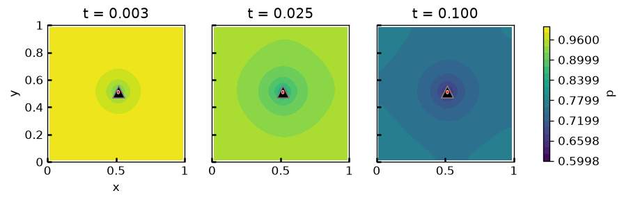
- "pressure": the depression cone grows (t = 0.003 → 0.025) and then stops changing shape, while the entire field subsides (t = 0.025 → 0.1). The colour scale is shared, so that late, uniform darkening is the decline.
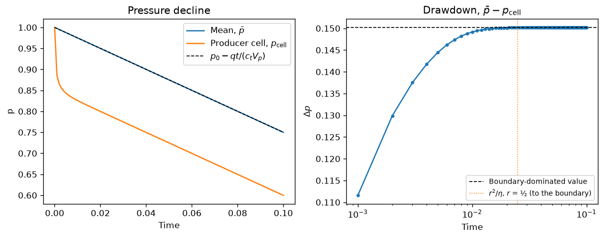
- "decline" (left): $\bar{p}$ falls exactly along the material-balance line (dashed), and the producer's cell pressure runs parallel to it, one drawdown below.
- "decline" (right): that drawdown (note the logarithmic time axis) grows throughout the transient, and then settles at 0.15 -- the transition occurring at about the time $r^2/η$ that the disturbance needs to reach the boundary (dotted).
Throughout, $p_\mathrm{cell}$ is the pressure of the cell that holds the well,
not that of the wellbore, so it deepens under grid refinement (0.15 at 32², 0.18
at 64²). For a bottom-hole pressure, give the well an rw and read
model.wells.actual_bhp instead; ref examples/well_control.py.
  1"""Primary depletion: production *without* injection.
  2
  3Impossible with `ct = 0` (the rates must balance, ref `Wells.rates`); with
  4`ct > 0` the deficit is drawn from *storage*, i.e. from the expansion of the
  5rock and fluids as the pressure drops.
  6
  7Two flow regimes are visible:
  8
  9- **Transient** (early): the pressure disturbance has not yet reached the
 10  (closed) boundaries, so the reservoir behaves as if it were infinite.
 11- **Boundary-dominated** (late): the disturbance has swept the whole domain, and
 12  the pressure profile is *frozen in shape* -- it simply subsides at the constant
 13  rate dictated by material balance,
 14
 15  $$ dp̄/dt = -q / (c_t V_p) $$
 16
 17  ($V_p$ = pore volume), and the drawdown $p̄ - p_\\mathrm{cell}$ is constant.
 18
 19There is no water anywhere here (`S = 0` throughout), so this is effectively a
 20single-phase example -- and, rates being signed (negative to produce),
 21the lone producer is the only well there is.
 22
 23In the figures:
 24
 25- "pressure": the depression cone grows (t = 0.003 → 0.025) and then stops
 26  changing shape, while the entire field subsides (t = 0.025 → 0.1).
 27  The colour scale is shared, so that late, uniform darkening *is* the decline.
 28- "decline" (left): $\\bar{p}$ falls exactly along the material-balance line
 29  (dashed), and the producer's *cell* pressure runs parallel to it, one drawdown
 30  below.
 31- "decline" (right): that drawdown (note the logarithmic time axis) grows
 32  throughout the transient, and then settles at 0.15 -- the transition
 33  occurring at about the time $r^2/η$ that the disturbance needs to reach the
 34  boundary (dotted).
 35
 36Throughout, $p_\\mathrm{cell}$ is the pressure of the *cell* that holds the well,
 37not that of the wellbore, so it deepens under grid refinement (0.15 at 32², 0.18
 38at 64²). For a bottom-hole pressure, give the well an `rw` and read
 39`model.wells.actual_bhp` instead; ref `examples/well_control.py`.
 40"""
 41
 42from mpl_tools.place import freshfig
 43import numpy as np
 44
 45from TPFA_ResSim import ResSim
 46from TPFA_ResSim.plotting import show
 47
 48## Setup
 49q = .25
 50model = ResSim(Lx=1, Ly=1, Nx=32, Ny=32, ct=.1,
 51               wells=[dict(xy=[.5, .5], rate=-q)])
 52
 53dt = 1e-3
 54nSteps = 100
 55tt = dt*np.arange(nSteps + 1)
 56oil_only = np.zeros(model.Nxy)
 57P0 = np.ones(model.Nxy)
 58
 59## Simulate
 60SS, PP = model.sim(dt, nSteps, oil_only, P0=P0, pbar=False)
 61assert SS.max() == 0, "No water is injected, so none should appear."
 62
 63iw = model.xy2ind(*model.wells.xy[0])
 64p_mean = PP.mean(axis=1)
 65p_cell = PP[:, iw]
 66pore_volume = model.h2 * model.por.sum()
 67
 68## Plot: the pressure field, subsiding
 69fig, axs = freshfig("Depletion -- pressure", ncols=3, sharex=True, sharey=True,
 70                    figsize=(9, 3.5))
 71kws: dict = dict(levels=np.linspace(PP.min(), 1, 21), cmap="viridis",
 72                 colorbar=False, finalize=False, wells=dict(size=.4))
 73for i, (ax, k) in enumerate(zip(axs, [3, 25, nSteps])):
 74    cc = model.plt_field(ax, PP[k], **kws, labels=(i == 0), title=f"t = {k*dt:.3f}")
 75fig.colorbar(cc, ax=axs, shrink=.6, label="p")
 76# Note how the *shape* stops changing, while the level keeps dropping.
 77
 78## Plot: decline and drawdown
 79fig, (ax1, ax2) = freshfig("Depletion -- decline", ncols=2, figsize=(10, 4))
 80
 81ax1.plot(tt, p_mean, label="Mean, $\\bar{p}$")
 82ax1.plot(tt, p_cell, label="Producer cell, $p_\\mathrm{cell}$")
 83ax1.plot(tt, 1 - q*tt/(model.ct*pore_volume), "k--", lw=1,
 84         label="$p_0 - q t / (c_t V_p)$")
 85ax1.set(title="Pressure decline", xlabel="Time", ylabel="p")
 86ax1.legend()
 87
 88ax2.plot(tt[1:], (p_mean - p_cell)[1:], "-o", ms=3)
 89ax2.set(title="Drawdown, $\\bar{p} - p_\\mathrm{cell}$", xlabel="Time",
 90        xscale="log", ylabel="$\\Delta p$")
 91ax2.axhline((p_mean - p_cell)[-1], c="k", ls="--", lw=1,
 92            label="Boundary-dominated value")
 93ax2.axvline(.25/(1/model.ct), c="C1", ls=":", lw=1,
 94            label="$r^2/η$, $r$ = ½ (to the boundary)")
 95ax2.legend(fontsize="small")
 96fig.tight_layout()
 97
 98# Material balance holds exactly (see also tests/test_compressible.py)
 99assert np.allclose(p_mean, 1 - q*tt/(model.ct*pore_volume))
100
101# Regression values, checked by `tests/test_examples.py`.
102__digest__ = dict(p_mean = p_mean,
103                  p_cell = p_cell,
104                  p_last = PP[-1])
105
106if __name__ == "__main__":
107    show()