examples
Runnable illustrations of the simulator.
Each is a plain, top-to-bottom script -- run as python examples/buildup.py, say --
whose docstring says what it shows, and whose figures are reproduced on its page here.
They double as regression tests: tests/test_examples.py runs them all
(plotting included) and compares the output with tests/references.py.
One panel per feature, drawn from their results:
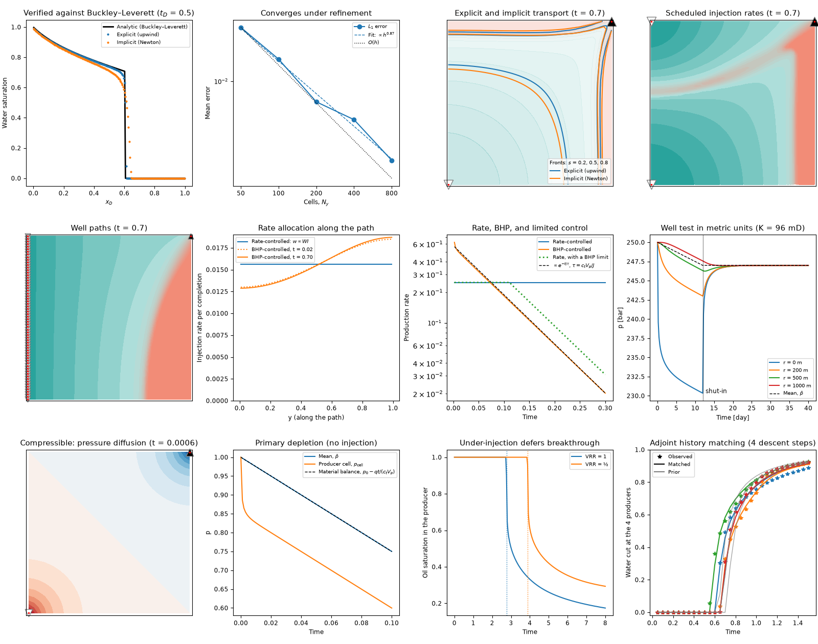
examples.heterogeneousandexamples.quarter_five_spotreproduce Figs. 1 and 6 of the reference paper. The latter is what verifies our agreement with the Matlab codes.examples.rate_schedulingsteers the water front using time-varying injection rates.examples.buckley_leverettis the only verification among them: in 1D the saturation equation is exactly solvable (by the Welge tangent construction), so here the numerical profile is compared with the truth rather than with ourselves, and the error is shown to vanish under grid refinement.
These concern the well model (TPFA_ResSim.wells.peaceman_WI), i.e. the sub-grid
relation between a well and the (much larger) cell that holds it:
examples.well_control: the two ways to control a well -- prescribing its rate and letting its pressure follow, or the reverse -- shown to be one model seen from either end. Also why the well model is needed at all: a well's cell pressure is a grid artefact, whereas the bottom-hole pressure derived from it is not.examples.well_path: a well completed along a polyline rather than in a single cell, and the two ways its rate then gets divided among the completions -- statically (in proportion to the well index) or, under BHP control, solved for.
The next ones illustrate what slight compressibility (TPFA_ResSim.ResSim.ct > 0) brings:
examples.pressure_diffusion: the pressure equation becomes parabolic, so that a change of rate propagates at finite speed (diffusivityη = K λ / (φ ct)), instead of being felt everywhere instantaneously. Also illustrates that the pressure level is now meaningful (anchored byp0), whereas the incompressible pressure is only defined up to a constant.examples.depletion: production without injection (impossible if incompressible), its transient and boundary-dominated regimes, and the resulting material-balance decline,dp̄/dt = -q / (ct Vp).examples.buildup: shutting in a well, and the ensuing pressure buildup. Monitor points far from the well respond late -- and keep declining after the shut-in, before turning around.examples.voidage_replacement: the only two-phase one of these -- waterflooding while injecting only half of what is produced (impossible if incompressible). The front then advances more slowly, and by a different pattern, since some of the oil is instead driven by expansion.
The last two illustrate the adjoint (TPFA_ResSim.tlm), i.e. gradients of an
objective wrt the initial state and the permeability field, checked against finite
differences:
examples.water_cut_gradient: the sensitivity of the producers' water cut.examples.history_match_gradient: a few steepest-descent steps towards a synthetic truth.
1"""Runnable illustrations of the simulator. 2 3Each is a plain, top-to-bottom script -- run as `python examples/buildup.py`, say -- 4whose docstring says what it shows, and whose figures are reproduced on its page here. 5 6They double as regression tests: `tests/test_examples.py` runs them all 7(plotting included) and compares the output with `tests/references.py`. 8 9One panel per feature, drawn from their results: 10 11 12 13- `examples.heterogeneous` and `examples.quarter_five_spot` reproduce Figs. 1 and 6 of 14 the reference paper. The latter is what verifies our agreement with the Matlab codes. 15- `examples.rate_scheduling` steers the water front using time-varying injection rates. 16- `examples.buckley_leverett` is the only *verification* among them: in 1D the 17 saturation equation is exactly solvable (by the Welge tangent construction), 18 so here the numerical profile is compared with the truth rather than with 19 ourselves, and the error is shown to vanish under grid refinement. 20 21These concern the *well model* (`TPFA_ResSim.wells.peaceman_WI`), i.e. the sub-grid 22relation between a well and the (much larger) cell that holds it: 23 24- `examples.well_control`: the two ways to control a well -- prescribing its rate and 25 letting its pressure follow, or the reverse -- shown to be one model seen from 26 either end. Also why the well model is needed at all: a well's *cell* pressure 27 is a grid artefact, whereas the bottom-hole pressure derived from it is not. 28- `examples.well_path`: a well completed along a polyline rather than in a single 29 cell, and the two ways its rate then gets divided among the completions -- 30 statically (in proportion to the well index) or, under BHP control, solved for. 31 32The next ones illustrate what slight compressibility (`TPFA_ResSim.ResSim.ct` > 0) brings: 33 34- `examples.pressure_diffusion`: the pressure equation becomes parabolic, so that a 35 change of rate propagates at *finite speed* (diffusivity `η = K λ / (φ ct)`), 36 instead of being felt everywhere instantaneously. Also illustrates that the 37 pressure level is now meaningful (anchored by `p0`), whereas the incompressible 38 pressure is only defined up to a constant. 39- `examples.depletion`: production *without* injection (impossible if incompressible), 40 its transient and boundary-dominated regimes, and the resulting material-balance 41 decline, `dp̄/dt = -q / (ct Vp)`. 42- `examples.buildup`: shutting in a well, and the ensuing pressure buildup. Monitor 43 points far from the well respond late -- and keep declining after the shut-in, 44 before turning around. 45- `examples.voidage_replacement`: the only *two-phase* one of these -- waterflooding 46 while injecting only half of what is produced (impossible if incompressible). 47 The front then advances more slowly, and by a different pattern, since some of 48 the oil is instead driven by expansion. 49 50The last two illustrate the adjoint (`TPFA_ResSim.tlm`), i.e. gradients of an 51objective wrt the initial state and the permeability field, checked against finite 52differences: 53 54- `examples.water_cut_gradient`: the sensitivity of the producers' water cut. 55- `examples.history_match_gradient`: a few steepest-descent steps towards a 56 synthetic truth. 57"""