examples.buckley_leverett
The Buckley--Leverett solution -- the one exact answer we can be checked against.
Every other example here is an illustration: we plot what the code does, and argue that it looks right. This one is a verification: in 1D, with constant total velocity, the water equation has an analytic solution (Buckley & Leverett, 1942), so the numerical profile can be compared with the truth, and the error made to shrink under refinement.
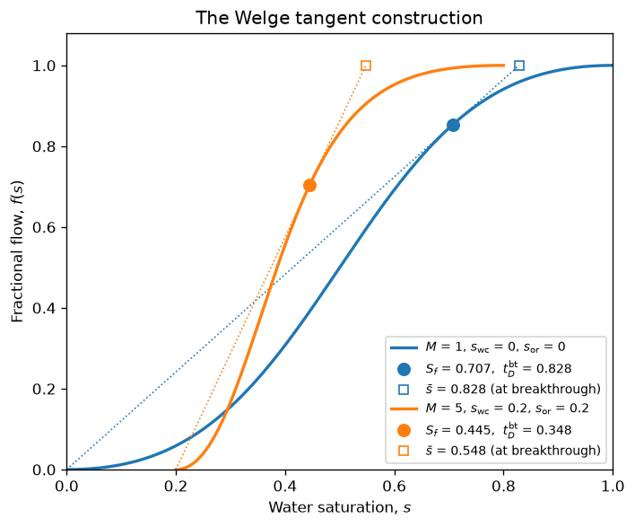
The construction. With $ ∇ ⋅ v = 0 $ the transport equation collapses to the scalar conservation law $$ φ \, ∂s/∂t + v \, ∂f(s)/∂x = 0 \,, $$ whose characteristics carry a given $s$ at speed $ v f'(s)/φ $. Since $f$ is S-shaped, $f'$ is not monotone, so those characteristics cross: the profile would become multivalued, and a shock forms instead. Its saturation, $S_f$, is fixed by requiring that the shock speed (from mass balance across it) equal the characteristic speed just behind it -- which is the Welge (1952) tangent construction: the chord from the initial state to $(S_f, f(S_f))$ must be tangent to $f$, $$ \frac{f(S_f)}{S_f - s_\mathrm{wc}} = f'(S_f) \,. $$ Everything else follows: the shock travels at that chord's slope, breakthrough occurs when it reaches the outlet, and thereafter the outlet saturation is read off $ f'(s) = 1/t_D $ (which is Welge's production forecast).
Closed form for this model. ResSim.RelPerm being quadratic, the tangent
condition can be solved by hand. In terms of the normalized saturation
(ref ResSim.rescale_sat) and the endpoint mobility ratio $ M = v_o/v_w $,
$$ S_f^* = \frac{1}{\sqrt{1 + M}} \,, \qquad
t_D^\mathrm{bt} = (1 - s_\mathrm{wc} - s_\mathrm{or})
\, \frac{2 \, (1 + M - \sqrt{1+M})}{M \, \sqrt{1+M}} \,, $$
so for the default unit-viscosity fluids $ S_f = 1/\sqrt{2} ≈ 0.7071 $ and
breakthrough comes at $ 2(\sqrt{2}-1) ≈ 0.8284 $ pore volumes injected. Below,
the tangent is located numerically (from the model's own RelPerm and
dRelPerm) and asserted to agree with these -- so the check cuts both ways:
it validates the analytic solution we then compare the simulation against.
Notes on the setup:
- Time is measured in pore volumes injected ($t_D$), and distance in fractions of the length ($x_D$). The rate, pore volume and length are all $1$ here, so $ t_D = t $ and $ x_D = y $ -- no scaling clutters the plots.
- The 1D domain is a single column of cells (
Nx=1), i.e. the flow is along $y$. A row (Ny=1) works just the same (tests/test_transport.pychecks that the two agree); the column is merely what the plots below assume. - The ends are wells (a source and a sink), not boundary conditions, which costs two $O(h)$ discrepancies with the textbook problem: the inlet cell only approaches $ s = 1 - s_\mathrm{or} $ (it is filled at a finite rate, not held at a value), and the outlet is sampled half a cell short of $ x_D = 1 $. Both are visible below, and both vanish under refinement.
In the figures:
- "fractional flow": the construction itself. The tangent from the initial state finds $ S_f = 0.71 $ for the unit-viscosity fluids, but only $0.44$ for the case with $ M = 5 $ -- a more adverse mobility ratio gives a weaker shock, arriving sooner (at $ t_D = 0.35 $ rather than $0.83$), which is the whole reason mobility ratio matters to a waterflood. Where the tangent reaches $ f = 1 $ (open squares) is Welge's second reading of it: the average saturation behind the front -- and hence, nothing having been produced yet, the recovery at breakthrough. Asserted against the simulation below.
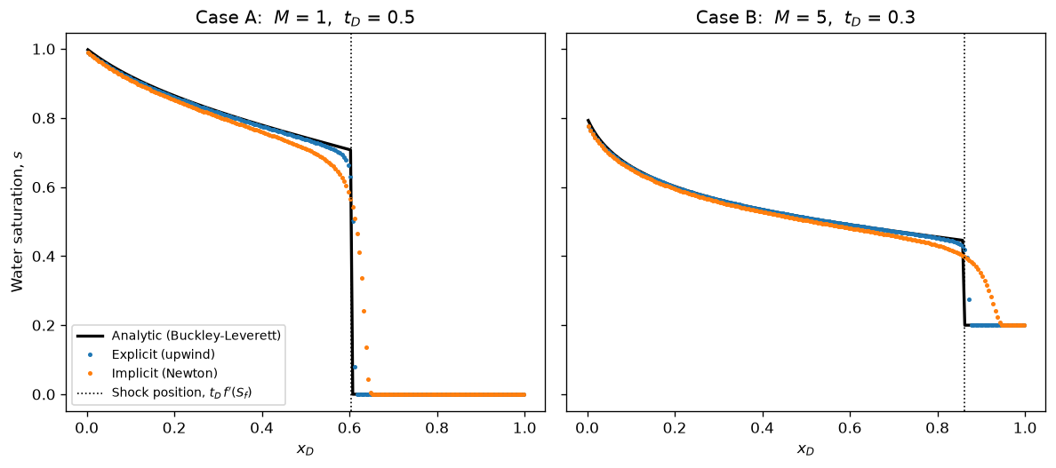
- "saturation profile": the numerical and analytic profiles, at a time before
breakthrough. The explicit scheme follows the rarefaction to within 0.017 in
saturation (0.005 on average), and smears the shock over some 4 cells. The
implicit scheme is four times as far off in the rarefaction, and spreads the
shock over five times as many cells -- as in
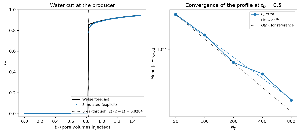
examples.quarter_five_spot, it is the more diffusive of the two. Note that neither overshoots. - "verification" (left): the water cut at the producer, against Welge's forecast. It breaks through a shade early (the producer being half a cell inside), then follows the analytic curve to within 0.004.
- "verification" (right): the $L_1$ error of the profile, which shrinks as $ h^{0.87} $ -- first-order convergence, all but the last 13% of it, the shortfall being the usual one for a monotone first-order scheme resolving a discontinuity. (The zig-zag about that fit is also expected: the error depends on where the shock happens to fall within a cell.) The rate is what matters: it certifies that the scheme is consistent, i.e. that the error is discretization, not bug.
  1"""The Buckley--Leverett solution -- the one *exact* answer we can be checked against.
  2
  3Every other example here is an *illustration*: we plot what the code does, and
  4argue that it looks right. This one is a **verification**: in 1D, with constant
  5total velocity, the water equation has an analytic solution
  6(Buckley & Leverett, 1942), so the numerical profile can be compared with the
  7truth, and the error made to shrink under refinement.
  8
  9**The construction.** With $ ∇ ⋅ v = 0 $ the transport equation collapses to the
 10scalar conservation law
 11$$ φ \\, ∂s/∂t + v \\, ∂f(s)/∂x = 0 \\,, $$
 12whose characteristics carry a given $s$ at speed $ v f'(s)/φ $. Since $f$ is
 13S-shaped, $f'$ is *not* monotone, so those characteristics cross: the profile
 14would become multivalued, and a **shock** forms instead. Its saturation,
 15$S_f$, is fixed by requiring that the shock speed (from mass balance across it)
 16equal the characteristic speed just behind it -- which is the **Welge (1952)
 17tangent** construction: the chord from the initial state to $(S_f, f(S_f))$ must
 18be tangent to $f$,
 19$$ \\frac{f(S_f)}{S_f - s_\\mathrm{wc}} = f'(S_f) \\,. $$
 20Everything else follows: the shock travels at that chord's slope, breakthrough
 21occurs when it reaches the outlet, and thereafter the outlet saturation is read
 22off $ f'(s) = 1/t_D $ (which is Welge's production forecast).
 23
 24**Closed form for this model.** `ResSim.RelPerm` being quadratic, the tangent
 25condition can be solved by hand. In terms of the normalized saturation
 26(ref `ResSim.rescale_sat`) and the endpoint mobility ratio $ M = v_o/v_w $,
 27$$ S_f^* = \\frac{1}{\\sqrt{1 + M}} \\,, \\qquad
 28   t_D^\\mathrm{bt} = (1 - s_\\mathrm{wc} - s_\\mathrm{or})
 29       \\, \\frac{2 \\, (1 + M - \\sqrt{1+M})}{M \\, \\sqrt{1+M}} \\,, $$
 30so for the default unit-viscosity fluids $ S_f = 1/\\sqrt{2} ≈ 0.7071 $ and
 31breakthrough comes at $ 2(\\sqrt{2}-1) ≈ 0.8284 $ pore volumes injected. Below,
 32the tangent is located *numerically* (from the model's own `RelPerm` and
 33`dRelPerm`) and asserted to agree with these -- so the check cuts both ways:
 34it validates the analytic solution we then compare the simulation against.
 35
 36Notes on the setup:
 37
 38- Time is measured in **pore volumes injected** ($t_D$), and distance in
 39  fractions of the length ($x_D$). The rate, pore volume and length are all
 40  $1$ here, so $ t_D = t $ and $ x_D = y $ -- no scaling clutters the plots.
 41- The 1D domain is a single **column** of cells (`Nx=1`), i.e. the flow is
 42  along $y$. A **row** (`Ny=1`) works just the same (`tests/test_transport.py`
 43  checks that the two agree); the column is merely what the plots below assume.
 44- The ends are **wells** (a source and a sink), not boundary conditions, which
 45  costs two $O(h)$ discrepancies with the textbook problem: the inlet cell only
 46  approaches $ s = 1 - s_\\mathrm{or} $ (it is filled at a finite rate, not
 47  held at a value), and the outlet is sampled half a cell short of $ x_D = 1 $.
 48  Both are visible below, and both vanish under refinement.
 49
 50In the figures:
 51
 52- "fractional flow": the construction itself. The tangent from the initial
 53  state finds $ S_f = 0.71 $ for the unit-viscosity fluids, but only $0.44$ for
 54  the case with $ M = 5 $ -- a *more adverse* mobility ratio gives a *weaker*
 55  shock, arriving sooner (at $ t_D = 0.35 $ rather than $0.83$), which is the
 56  whole reason mobility ratio matters to a waterflood. Where the tangent
 57  reaches $ f = 1 $ (open squares) is Welge's second reading of it: the
 58  *average* saturation behind the front -- and hence, nothing having been
 59  produced yet, the recovery at breakthrough. Asserted against the simulation
 60  below.
 61- "saturation profile": the numerical and analytic profiles, at a time before
 62  breakthrough. The explicit scheme follows the rarefaction to within 0.017 in
 63  saturation (0.005 on average), and smears the shock over some 4 cells. The
 64  implicit scheme is four times as far off in the rarefaction, and spreads the
 65  shock over five times as many cells -- as in `examples.quarter_five_spot`, it is
 66  the more diffusive of the two. Note that neither *overshoots*.
 67- "verification" (left): the water cut at the producer, against Welge's
 68  forecast. It breaks through a shade early (the producer being half a cell
 69  inside), then follows the analytic curve to within 0.004.
 70- "verification" (right): the $L_1$ error of the profile, which shrinks as
 71  $ h^{0.87} $ -- first-order convergence, all but the last 13% of it, the
 72  shortfall being the usual one for a monotone first-order scheme resolving a
 73  discontinuity. (The zig-zag about that fit is also expected: the error
 74  depends on where the shock happens to fall within a cell.) The rate is what
 75  matters: it certifies that the scheme is consistent, i.e. that the error is
 76  *discretization*, not *bug*.
 77"""
 78
 79from mpl_tools.place import freshfig
 80import numpy as np
 81from scipy.optimize import minimize_scalar
 82
 83from TPFA_ResSim import ResSim
 84from TPFA_ResSim.plotting import show
 85
 86## Setup
 87
 88
 89def make_model(N: int, fluid: dict) -> ResSim:
 90    """A 1D column of `N` cells: injector at the bottom, producer at the top.
 91
 92    Unit length, unit pore volume, unit rate -- so that time *is* $t_D$
 93    (pore volumes injected), and position *is* $x_D$.
 94    """
 95    return ResSim(Lx=1, Ly=1, Nx=1, Ny=N, **fluid,
 96                  wells=[dict(xy=[0, 0], rate=+1),
 97                         dict(xy=[0, 1], rate=-1)])
 98
 99
100## The analytic solution
101# NB: built from the model's *own* `RelPerm`/`dRelPerm`, so that it cannot
102# drift from the simulator's notion of the fluids -- only from its numerics.
103
104
105def frac_flow(model, s):
106    """Fractional flow of water, $ f = λ_w / (λ_w + λ_o) $."""
107    Mw, Mo = model.RelPerm(s)
108    return Mw / (Mw + Mo)
109
110
111def d_frac_flow(model, s):
112    """Derivative $ f'(s) $, i.e. the speed of the characteristic carrying `s`."""
113    Mw, Mo = model.RelPerm(s)
114    dMw, dMo = model.dRelPerm(s)
115    return (dMw*Mo - Mw*dMo) / (Mw + Mo)**2
116
117
118def welge_tangent(model) -> tuple:
119    """Locate the shock: `(S_f, shock speed)`, ref the docstring.
120
121    Rather than solving $ f(S)/(S - s_\\mathrm{wc}) = f'(S) $, we *maximize*
122    the chord slope -- the same point, but needing no derivative, and with no
123    root-bracketing to get wrong.
124    """
125    lo, hi = model.swc, 1 - model.sor
126    chord = lambda S: frac_flow(model, S) / (S - lo)  # noqa: E731
127    opt = minimize_scalar(lambda S: -chord(S), method="bounded",
128                          bounds=(lo + 1e-9, hi), options=dict(xatol=1e-12))
129    return opt.x, chord(opt.x)
130
131
132def analytic(model, tD, xD, S_f):
133    """The saturation at `xD` at time `tD`: the profile, and its shock.
134
135    Behind the shock, $ x_D = t_D \\, f'(s) $ -- monotone in $s$ over
136    $ [S_f, 1 - s_\\mathrm{or}] $ (the tangent point lying beyond $f$'s
137    inflection), so it is inverted by interpolation. The shock itself needs no
138    special treatment: the tangent condition puts its position at exactly the
139    end of that range, so anything ahead of it is simply `right=swc`.
140    """
141    ss = np.linspace(S_f, 1 - model.sor, 10001)
142    xx = tD * d_frac_flow(model, ss)
143    return np.interp(xD, xx[::-1], ss[::-1], right=model.swc)
144
145
146## Verify the analytic solution against the closed form
147cases: dict = dict(
148    A=dict(),                              # defaults: vw = vo = 1, swc = sor = 0
149    B=dict(vo=5., swc=.2, sor=.2),         # a contrast in both viscosity and endpoints
150)
151
152models = {case: make_model(200, fluid) for case, fluid in cases.items()}
153
154for case, model in models.items():
155    S_f, speed = welge_tangent(model)
156    # The closed form (ref the docstring), in terms of `M` and the endpoints
157    M = model.vo / model.vw
158    span = 1 - model.swc - model.sor
159    S_f_exact = model.swc + span / np.sqrt(1 + M)
160    tD_bt_exact = span * 2*(1 + M - np.sqrt(1 + M)) / (M * np.sqrt(1 + M))
161    assert np.isclose(S_f, S_f_exact, rtol=1e-8), "Welge tangent misplaced."
162    assert np.isclose(1/speed, tD_bt_exact, rtol=1e-8), "Closed form disagrees."
163    print(f"Case {case}: M = {M:g}, S_f = {S_f:.4f}, breakthrough at {1/speed:.4f} PVI")
164
165## Simulate: the profile, both schemes, both cases
166tD_snap = dict(A=.5, B=.3)  # a time before breakthrough, for each case
167profiles: dict = {}
168
169for case, model in models.items():
170    S_f, speed = welge_tangent(model)
171    xD = model.mesh[1].ravel()
172    S0 = np.full(model.Nxy, model.swc)
173
174    nSteps = 50
175    dt = tD_snap[case] / nSteps
176    S_exp, _ = model.sim(dt, nSteps, S0, pbar=False)
177    S_imp, _ = model.sim(dt, nSteps, S0, pbar=False, implicit=True)
178
179    profiles[case] = dict(xD=xD, S_f=S_f, speed=speed,
180                          exact=analytic(model, tD_snap[case], xD, S_f),
181                          explicit=S_exp[-1], implicit=S_imp[-1])
182
183    # Neither scheme may overshoot the physical range: the analytic solution is
184    # bounded by its data, and a monotone scheme must be too.
185    for scheme, S in [("explicit", S_exp), ("implicit", S_imp)]:
186        assert model.swc - 1e-12 <= S.min() and S.max() <= 1 - model.sor + 1e-12, (
187            f"Case {case}, {scheme} scheme: saturation out of bounds.")
188
189## Simulate: the production history (case A, past breakthrough)
190model = models["A"]
191S_f, speed = welge_tangent(model)
192tD_bt = 1 / speed
193
194nSteps = 150
195dt = 1.5 / nSteps
196tt = dt * np.arange(nSteps + 1)
197SS, _ = model.sim(dt, nSteps, np.full(model.Nxy, model.swc), pbar=False)
198
199# The water cut is the fractional flow of the producer's cell -- ref
200# `ResSim.assemble_wells`, which is what draws the produced fluid at that ratio.
201i_prd = model.xy2ind(*model.wells.xy[1])
202water_cut = frac_flow(model, SS[:, i_prd])
203# Welge's forecast: the outlet saturation is the one whose characteristic has
204# just arrived. `analytic` returns `swc` (whence a zero water cut) before that.
205water_cut_exact = np.array([frac_flow(model, analytic(model, t, 1., S_f))
206                            for t in tt])
207water_cut_exact[0] = 0  # `tD = 0` puts the whole profile at the inlet
208
209# Mass balance: what was injected is either still in place, or was produced.
210# (The tolerance is set by the trapezoidal integration of the jump at
211# breakthrough, not by the scheme, which conserves mass exactly.)
212in_place = (SS[-1] - model.swc).mean()
213produced = np.trapezoid(water_cut, tt)
214assert np.isclose(in_place + produced, tt[-1], rtol=2e-3), "Water unaccounted for."
215
216# Before breakthrough that balance is *exact*, nothing having been produced.
217# NB: "nothing" is not quite `0`: the explicit scheme's stencil advances one
218# cell per sub-step, so a (multiplicatively vanishing) tail of the front runs
219# ahead of it -- reaching the producer at some $ 10^{-150} $, long before the
220# water does. Hence the threshold, which also defines breakthrough below.
221DRY = 1e-4  # water cut counting as "no water", i.e. $ s ⪅ 0.01 $
222k_pre = round(.7 / dt)
223assert water_cut[k_pre] < DRY, "Breakthrough far too early."
224assert np.isclose((SS[k_pre] - model.swc).mean(), tt[k_pre]), "Injected water lost."
225
226# Breakthrough should be *slightly* early, the producer sitting half a cell
227# short of the outlet -- i.e. by `(hy/2) / speed`, which is under one `dt` here.
228tD_bt_sim = tt[(water_cut > DRY).argmax()]
229assert 0 <= tD_bt - tD_bt_sim < 2*dt, "Breakthrough mistimed."
230
231# Evaluated at breakthrough, it is the *other* reading of the tangent (ref the
232# "fractional flow" figure): the mean saturation is then the average behind the
233# front, $ s_wc + t_D^bt $ -- to within the smearing.
234k_bt = round(tD_bt / dt)
235assert np.isclose(SS[k_bt].mean(), model.swc + tD_bt, rtol=1e-2), (
236    "Welge average is off.")
237
238## Simulate: convergence under refinement (case A, explicit scheme)
239NN = np.array([50, 100, 200, 400, 800])
240L1 = np.zeros(len(NN))
241
242for i, N in enumerate(NN):
243    m = make_model(N, cases["A"])
244    S, _ = m.sim(tD_snap["A"]/50, 50, np.full(m.Nxy, m.swc), pbar=False)
245    # NB: the analytic solution is grid-independent -- only sampled anew
246    exact = analytic(m, tD_snap["A"], m.mesh[1].ravel(), profiles["A"]["S_f"])
247    L1[i] = abs(S[-1] - exact).mean()
248
249fit = np.polyfit(np.log(NN), np.log(L1), 1)
250rate = -fit[0]
251print(f"Convergence: L1 error ~ h^{rate:.2f}")
252assert .7 < rate < 1.1, "Lost (near-)first-order convergence."
253
254## Plot: the fractional-flow curve and the Welge tangent
255fig, ax = freshfig("Buckley-Leverett -- fractional flow", figsize=(6, 5))
256
257for case, p in profiles.items():
258    m = models[case]
259    S_f, tD_bt_ = p["S_f"], 1 / p["speed"]
260    ss = np.linspace(m.swc, 1 - m.sor, 201)
261    (h,) = ax.plot(ss, frac_flow(m, ss), lw=2,
262                   label=f"$M$ = {m.vo/m.vw:g}, "
263                         f"$s_\\mathrm{{wc}}$ = {m.swc:g}, "
264                         f"$s_\\mathrm{{or}}$ = {m.sor:g}")
265    # The tangent, from the initial state up to `f = 1`, which it reaches at
266    # the *average* saturation behind the front (Welge's other reading of it).
267    ax.plot([m.swc, m.swc + tD_bt_], [0, 1], ":", c=h.get_color(), lw=1)
268    ax.plot(S_f, frac_flow(m, S_f), "o", c=h.get_color(), ms=8,
269            label=f"$S_f$ = {S_f:.3f},  $t_D^\\mathrm{{bt}}$ = {tD_bt_:.3f}")
270    ax.plot(m.swc + tD_bt_, 1, "s", c=h.get_color(), ms=6, mfc="none",
271            label=f"$\\bar{{s}}$ = {m.swc + tD_bt_:.3f} (at breakthrough)")
272
273ax.set(title="The Welge tangent construction", xlabel="Water saturation, $s$",
274       ylabel="Fractional flow, $f(s)$", xlim=(0, 1), ylim=(0, 1.08))
275ax.legend(fontsize="small", loc="lower right")
276fig.tight_layout()
277
278## Plot: the saturation profiles, numerical vs. analytic
279fig, axs = freshfig("Buckley-Leverett -- saturation profile", ncols=2,
280                    sharey=True, figsize=(10, 4.5))
281
282for ax, (case, p) in zip(axs, profiles.items()):
283    ax.plot(p["xD"], p["exact"], "k-", lw=2, label="Analytic (Buckley-Leverett)")
284    ax.plot(p["xD"], p["explicit"], "C0.", ms=4, label="Explicit (upwind)")
285    ax.plot(p["xD"], p["implicit"], "C1.", ms=4, label="Implicit (Newton)")
286    ax.axvline(tD_snap[case] * p["speed"], c="k", ls=":", lw=1,
287               label="Shock position, $t_D \\, f'(S_f)$")
288    m = models[case]
289    ax.set(title=f"Case {case}:  $M$ = {m.vo/m.vw:g},"
290                 f"  $t_D$ = {tD_snap[case]}", xlabel="$x_D$")
291axs[0].set_ylabel("Water saturation, $s$")
292axs[0].legend(fontsize="small")
293fig.tight_layout()
294
295## Plot: water cut, and the convergence of the profile
296fig, (ax1, ax2) = freshfig("Buckley-Leverett -- verification", ncols=2,
297                           figsize=(10, 4.5))
298
299ax1.plot(tt, water_cut_exact, "k-", lw=2, label="Welge forecast")
300ax1.plot(tt, water_cut, "C0.", ms=4, label="Simulated (explicit)")
301ax1.axvline(tD_bt, c="k", ls=":", lw=1,
302            label=f"Breakthrough, $2(\\sqrt{{2}}-1)$ = {tD_bt:.4f}")
303ax1.set(title="Water cut at the producer", xlabel="$t_D$ (pore volumes injected)",
304        ylabel="$f_w$", ylim=(-.03, 1))
305ax1.legend(fontsize="small", loc="lower right")
306
307ax2.loglog(NN, L1, "C0-o", label="$L_1$ error")
308ax2.loglog(NN, np.exp(np.polyval(fit, np.log(NN))), "C0--", lw=1,
309           label=f"Fit: $\\propto h^{{{rate:.2f}}}$")
310ax2.loglog(NN, L1[0] * NN[0]/NN, "k:", lw=1, label="$O(h)$, for reference")
311ax2.set(title=f"Convergence of the profile at $t_D$ = {tD_snap['A']}",
312        xlabel="$N_y$", ylabel="Mean $|s - s_\\mathrm{exact}|$",
313        xticks=NN, xticklabels=[str(N) for N in NN])
314ax2.minorticks_off()
315ax2.legend(fontsize="small")
316fig.tight_layout()
317
318# Regression values, checked by `tests/test_examples.py`.
319__digest__ = dict(explicit  = profiles["A"]["explicit"],
320                  implicit  = profiles["A"]["implicit"],
321                  case_B    = profiles["B"]["explicit"],
322                  welge     = [profiles[c][k] for c in "AB"
323                               for k in ["S_f", "speed"]],
324                  water_cut = water_cut[water_cut > DRY],
325                  bt        = [tD_bt_sim, tD_bt],
326                  L1        = L1)
327
328if __name__ == "__main__":
329    show()