examples.quarter_five_spot
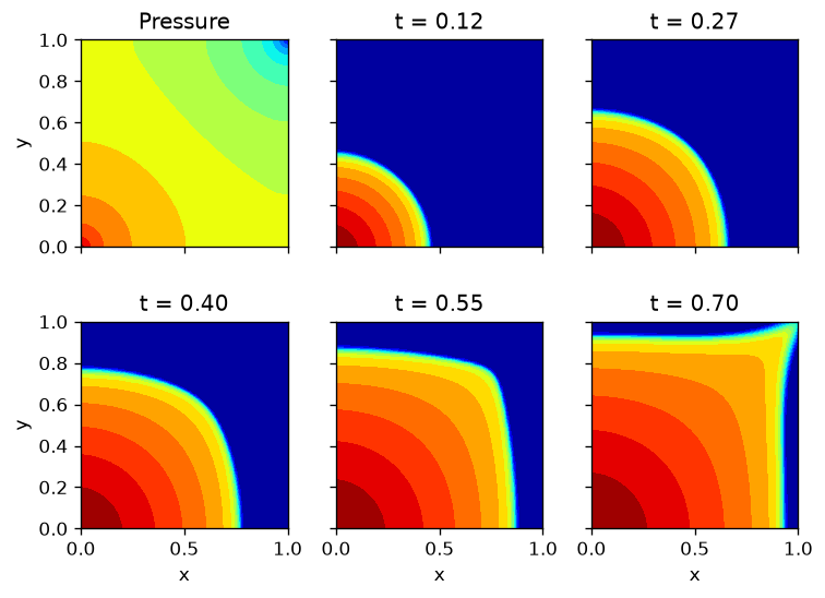
Reproduce Fig. 6 of the reference paper, i.e. listing 9.
This runs the familiar 5-spot well pattern on a homogeneous and isotropic permeability which, thanks to symmetry, only requires computing one of the 4 quadrants, giving it the quarter-five spot problem.
There are some minor discrepancies compared with their Fig. 6.
- They claim to plot the initial pressure, but it rather seems like the final one to me.
- They panels portray
tvalues are not available from the chosen time steps. - Their water front has a corner that is more protruding (not due to the previous issue).
However, since we generate the very same output as the matlab code, we believe the issue lies with the description in the paper, not with any error in the code.
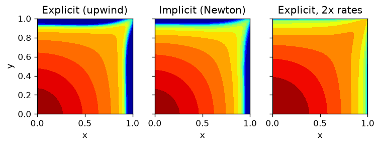
The last figure compares the two transport schemes (whose outputs are both verified against matlab) as well as a doubled-rate run.
In the figures:
- "Fig. 6": the water, injected in the SW corner, advances on the producer in the NE, in the shape that gives the quarter five-spot its name -- essentially that of the isobars of the first panel.
- "final saturation": the implicit scheme is the more diffusive of the two: its transition band ($0.2 < S < 0.8$) is some 15% wider than the explicit one's. Doubling the rates, meanwhile, simply gets further in the same time (mean saturation 0.86, against 0.70).
  1"""Reproduce Fig. 6 of the reference paper, i.e. listing 9.
  2
  3This runs the familiar 5-spot well pattern on a homogeneous and isotropic permeability
  4which, thanks to symmetry, only requires computing one of the 4 quadrants,
  5giving it the quarter-five spot problem.
  6
  7There are some minor discrepancies compared with their Fig. 6.
  8
  9- They claim to plot the initial pressure, but it rather seems like the final one to me.
 10- They panels portray `t` values are not available from the chosen time steps.
 11- Their water front has a corner that is more protruding (not due to the previous issue).
 12
 13However, since we generate the very same output as the matlab code, we believe
 14the issue lies with the description in the paper, not with any error in the code.
 15
 16The last figure compares the two transport schemes (whose outputs are both
 17verified against matlab) as well as a doubled-rate run.
 18
 19In the figures:
 20
 21- "Fig. 6": the water, injected in the SW corner, advances on the producer in
 22  the NE, in the shape that gives the quarter five-spot its name -- essentially
 23  that of the isobars of the first panel.
 24- "final saturation": the implicit scheme is the more diffusive of the two: its
 25  transition band ($0.2 < S < 0.8$) is some 15% wider than the explicit one's.
 26  Doubling the rates, meanwhile, simply gets further in the same time
 27  (mean saturation 0.86, against 0.70).
 28"""
 29
 30from mpl_tools.place import freshfig
 31import numpy as np
 32
 33from TPFA_ResSim import ResSim
 34from TPFA_ResSim.plotting import show
 35
 36## Setup
 37grid: dict = dict(Lx=1, Ly=1, Nx=64, Ny=64)
 38# Fluid properties are left at their defaults: vw = vo = 1, swc = sor = 0.
 39
 40
 41def wells(q):
 42    """A well is a record of its position and its (signed) rate.
 43
 44    Ref `ResSim.wells`. Here: an injector (SW) and a producer (NE).
 45    """
 46    return [dict(xy=[0, 0], rate=+q),
 47            dict(xy=[1, 1], rate=-q)]
 48
 49
 50
 51model = ResSim(**grid, wells=wells(1))
 52model_2x = ResSim(**grid, wells=wells(2))
 53
 54water_sat0 = model.swc * np.ones(model.Nxy)
 55nSteps = 28
 56dt = 0.7/nSteps
 57
 58## Simulate
 59SS_exp, PP_exp = model.sim(dt, nSteps, water_sat0, pbar=False)
 60SS_imp, PP_imp = model.sim(dt, nSteps, water_sat0, implicit=True, pbar=False)
 61SS_2x , PP_2x  = model_2x.sim(dt, nSteps, water_sat0, pbar=False)
 62
 63## Plot: the paper's Fig. 6 (from the explicit scheme)
 64kws = dict(levels=17, cmap="jet", origin=None, extent=(0, model.Lx, 0, model.Ly))
 65
 66fig, axs = freshfig("Fig. 6", nrows=2, ncols=3, sharex=True, sharey=True,
 67                    subplot_kw={'aspect': 'equal'})
 68
 69for ax, t in zip(axs.ravel(), [None, .14, .28, .42, .56, .70]):
 70    if ax.get_subplotspec().is_last_row() : ax.set_xlabel("x")  # noqa
 71    if ax.get_subplotspec().is_first_col(): ax.set_ylabel("y")  # noqa
 72
 73    if t is None:
 74        ax.set_title("Pressure")
 75        [P, V] = model.pressure_step(SS_exp[-1])  # Final+1 pressure
 76        ax.contourf(P.reshape(model.shape).T, **kws)
 77
 78    else:
 79        k = int(t/dt)
 80        ax.set_title("t = {:.2f}".format(k * dt))
 81        Z = SS_exp[k].reshape(model.shape).T  # transpose/flip for plot orientation
 82
 83        # Puts the values in gridcell centers (agrees w/ finite-vol. interpretation)
 84        # ax.imshow(Z[::-1], **kws)
 85
 86        # Also colocates with gridcell centers, but does not extend to edges.
 87        # ax.contourf(Z, levels=17, cmap="jet", origin="lower")
 88
 89        # Artificially stretches the field
 90        ax.contourf(Z, **kws)
 91
 92fig.tight_layout()
 93
 94## Plot: scheme and rate comparison (at the final time)
 95fig, axs = freshfig("Quarter five-spot -- final saturation", ncols=3,
 96                    sharex=True, sharey=True, subplot_kw={'aspect': 'equal'})
 97
 98for ax, (S, title) in zip(axs, [(SS_exp[-1], "Explicit (upwind)"),
 99                                (SS_imp[-1], "Implicit (Newton)"),
100                                (SS_2x[-1] , "Explicit, 2x rates")]):
101    ax.set_title(title)
102    ax.set_xlabel("x")
103    ax.contourf(S.reshape(model.shape).T, **kws)
104axs[0].set_ylabel("y")
105# The implicit scheme is (as usual) the more diffusive: its front is smeared.
106
107fig.tight_layout()
108
109## Animation
110prod = [model.xy2ind(*model.wells.xy[1])]
111animation = model.anim(SS_exp, SS_exp[1:, prod])
112
113# Regression values, checked by `tests/test_examples.py`.
114# The sub-sampling `[::600]` matches that of the matlab reference values.
115__digest__ = dict(explicit = SS_exp[-1, ::600],
116                  implicit = SS_imp[-1, ::600],
117                  doubled  = SS_2x[-1, ::600])
118
119if __name__ == "__main__":
120    show()