examples.rate_scheduling
Steering the water front with time-varying injection rates.
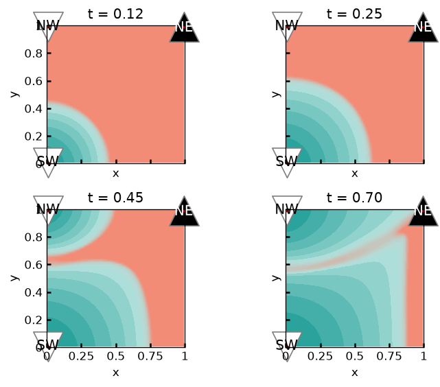
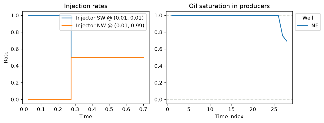
Two injectors (SW and NW corners) feed a single producer (NE corner). Their rates are scheduled: for the first 10 steps all of the water enters from the SW corner, thereafter the two injectors share the load equally. The resulting front is correspondingly lopsided.
A rate may be specified as a schedule (an array over time), as done here --
whereupon the wells held constant get broadcast along with it -- or (for
feedback control, e.g. shutting wells on water breakthrough) by overriding
ResSim.well_controls.
In the figures:
- "saturation": at t = 0.125, and still at t = 0.25 (the moment of the switch),
all of the water has come from the SW. By t = 0.45 a second front has grown
from the NW injector, and by t = 0.70 the two have merged into a distinctly
lopsided sweep -- compare the symmetric front of
examples.quarter_five_spot. - "wells": the schedule itself (left), and the oil saturation in the producer (right), which shows that the water only breaks through at the very end (step 27 of 28).
 1"""Steering the water front with time-varying injection rates.
 2
 3Two injectors (SW and NW corners) feed a single producer (NE corner).
 4Their rates are *scheduled*: for the first 10 steps all of the water enters from
 5the SW corner, thereafter the two injectors share the load equally.
 6The resulting front is correspondingly lopsided.
 7
 8A rate may be specified as a *schedule* (an array over time), as done here --
 9whereupon the wells held constant get broadcast along with it -- or (for
10feedback control, e.g. shutting wells on water breakthrough) by overriding
11`ResSim.well_controls`.
12
13In the figures:
14
15- "saturation": at t = 0.125, and still at t = 0.25 (the moment of the switch),
16  all of the water has come from the SW. By t = 0.45 a second front has grown
17  from the NW injector, and by t = 0.70 the two have merged into a distinctly
18  lopsided sweep -- compare the symmetric front of `examples.quarter_five_spot`.
19- "wells": the schedule itself (left), and the oil saturation in the producer
20  (right), which shows that the water only breaks through at the very end
21  (step 27 of 28).
22"""
23
24from mpl_tools.place import freshfig
25import numpy as np
26
27from TPFA_ResSim import ResSim
28from TPFA_ResSim.plotting import show
29
30## Setup
31nSteps = 28
32dt = 0.7/nSteps
33
34# Schedule: the SW injector carries everything until step 10, then they share.
35rate_sw = .5*np.ones(nSteps)
36rate_nw = .5*np.ones(nSteps)
37rate_sw[:10] = 1
38rate_nw[:10] = 0
39
40model = ResSim(Lx=1, Ly=1, Nx=64, Ny=64, wells=[
41    dict(name="SW", xy=[0, 0], rate=+rate_sw),
42    dict(name="NW", xy=[0, 1], rate=+rate_nw),
43    dict(name="NE", xy=[1, 1], rate=-1),   # constant: broadcast to the schedule
44])
45
46water_sat0 = model.swc * np.ones(model.Nxy)
47
48## Simulate
49SS, PP = model.sim(dt, nSteps, water_sat0, pbar=False)
50
51## Plot: saturation snapshots
52fig, axs = freshfig("Rate scheduling -- saturation", nrows=2, ncols=2,
53                    sharex=True, sharey=True)
54for ax, k in zip(axs.ravel(), [5, 10, 18, nSteps]):
55    model.plt_field(ax, SS[k], "oil", finalize=False, colorbar=False,
56                    title=f"t = {k*dt:.2f}")
57fig.tight_layout()
58
59## Plot: the schedule itself, and the resulting production
60fig, axs = freshfig("Rate scheduling -- wells", ncols=2, figsize=(9, 3.5))
61
62tt = dt*(1 + np.arange(nSteps))
63for i, rate in enumerate(model.wells.actual_rates[:2]):
64    x, y = model.wells.xy[i]
65    name = model.wells.names[i]
66    axs[0].step(tt, rate, where="post", label=f"Injector {name} @ ({x:.2f}, {y:.2f})")
67axs[0].set(title="Injection rates", xlabel="Time", ylabel="Rate", ylim=(-.05, 1.05))
68axs[0].legend()
69
70prd = [model.xy2ind(*model.wells.xy[2])]
71model.plt_production(axs[1], SS[1:, prd], finalize=False,
72                     labels=model.wells.names[2:])
73fig.tight_layout()
74
75# Regression values, checked by `tests/test_examples.py`.
76__digest__ = dict(sat_final=SS[-1, ::600])
77
78if __name__ == "__main__":
79    show()