examples.history_match_gradient
The gradient of a production-history misfit wrt. $\log K$, and a few descent steps.
The history-matching case, in its simplest form. A truth permeability field
(smoothed, log-normal) produces the observations: the water cut at each of
the four producers of a five-spot, at every time step. The prior guess is
homogeneous, $\log K = 0$. The objective is the mean squared error of the
prior's production history against the observations, and
TPFA_ResSim.tlm.adjoint gives its gradient with respect to every cell's
$\log K$ -- checked against a finite difference in a random direction -- for
about the cost of one more simulation, however many cells there are. That is
what makes gradient-based history matching feasible at all, and a few steps of
steepest descent (each with a coarse line search) are taken to show it works:
the misfit falls, and the update goes the way of the truth.
The seeds are those of a data misfit
(ref the "Seeding" section of TPFA_ResSim.tlm): for each observed time and
producer, the residual, weighted by the derivative of the observation operator
-- here $ f_w'(s) $ in the producer's cell, via tlm.fractional_flow.
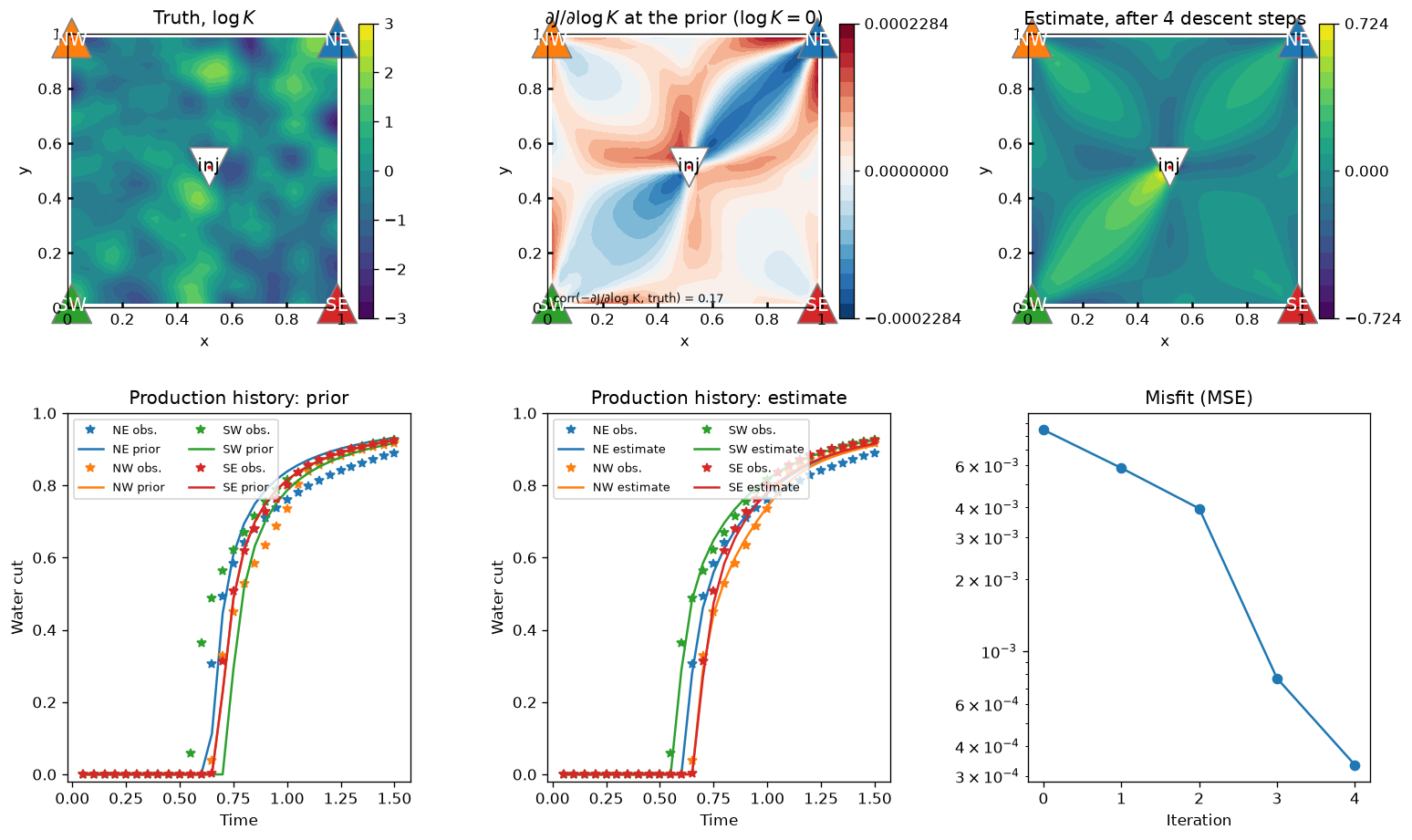
In the figure:
- Top left: the truth $\log K$, which the observations come from.
- Top middle: the gradient of the misfit at the prior. Since the prior is homogeneous, this is the whole of the first update (with a minus sign): it is negative (raise $K$) where the truth is permeable and the water reaches a producer through it, positive where the truth is tight -- but only where the production data are sensitive, i.e. along the flow paths. Hence its correlation with the truth over the whole field is weak (about 0.2; it is recorded in the digest): the data are blind to most of the field.
- Top right: the estimate after the descent steps (on its own colour scale: the update is far smaller than the truth's variations). It moves towards the truth along the flow paths and not elsewhere, the data saying nothing about the rest: the classic ill-posedness that a prior (regularization) would address.
- Bottom: the production histories -- observations, prior, and the final estimate -- and the misfit per iteration.
Steepest descent is used for its simplicity, not its merit.
A Gauss--Newton or quasi-Newton method, and a prior term, would do far better; the point here is the gradient, which any of them needs.
  1"""The gradient of a production-history misfit wrt. $\\log K$, and a few descent steps.
  2
  3The history-matching case, in its simplest form. A *truth* permeability field
  4(smoothed, log-normal) produces the *observations*: the water cut at each of
  5the four producers of a five-spot, at every time step. The *prior* guess is
  6homogeneous, $\\log K = 0$. The objective is the mean squared error of the
  7prior's production history against the observations, and
  8`TPFA_ResSim.tlm.adjoint` gives its gradient with respect to every cell's
  9$\\log K$ -- checked against a finite difference in a random direction -- for
 10about the cost of one more simulation, however many cells there are. That is
 11what makes gradient-based history matching feasible at all, and a few steps of
 12steepest descent (each with a coarse line search) are taken to show it works:
 13the misfit falls, and the update goes the way of the truth.
 14
 15The seeds are those of a data misfit
 16(ref the "Seeding" section of `TPFA_ResSim.tlm`): for each observed time and
 17producer, the residual, weighted by the derivative of the observation operator
 18-- here $ f_w'(s) $ in the producer's cell, via `tlm.fractional_flow`.
 19
 20In the figure:
 21
 22- Top left: the truth $\\log K$, which the observations come from.
 23- Top middle: the gradient of the misfit at the prior. Since the prior is
 24  homogeneous, this is the whole of the first update (with a minus sign): it
 25  is negative (raise $K$) where the truth is permeable *and* the water reaches
 26  a producer through it, positive where the truth is tight -- but only where
 27  the production data are sensitive, i.e. along the flow paths. Hence its
 28  correlation with the truth over the whole field is weak (about 0.2; it is
 29  recorded in the digest): the data are blind to most of the field.
 30- Top right: the estimate after the descent steps (on its own colour scale:
 31  the update is far smaller than the truth's variations). It moves towards
 32  the truth along the flow paths and not elsewhere, the data saying nothing
 33  about the rest: the classic ill-posedness that a prior (regularization)
 34  would address.
 35- Bottom: the production histories -- observations, prior, and the final
 36  estimate -- and the misfit per iteration.
 37
 38.. note:: Steepest descent is used for its simplicity, not its merit.
 39
 40    A Gauss--Newton or quasi-Newton method, and a prior term, would do far
 41    better; the point here is the *gradient*, which any of them needs.
 42"""
 43
 44from mpl_tools.place import freshfig
 45import numpy as np
 46from scipy.ndimage import uniform_filter as smooth
 47
 48from TPFA_ResSim import ResSim
 49from TPFA_ResSim.plotting import show
 50from TPFA_ResSim.tlm import adjoint, fractional_flow
 51
 52rng = np.random.default_rng(1)  # Reproducibility (the values are regression tested)
 53
 54## Model: a five-spot
 55wells = [
 56    dict(xy=[.5, .5], rate=+1  , name="inj"),
 57    dict(xy=[1 , 1 ], rate=-.25, name="NE"),
 58    dict(xy=[0 , 1 ], rate=-.25, name="NW"),
 59    dict(xy=[0 , 0 ], rate=-.25, name="SW"),
 60    dict(xy=[1 , 0 ], rate=-.25, name="SE"),
 61]
 62grid: dict = dict(Lx=1, Ly=1, Nx=32, Ny=32)
 63dt, nSteps = .05, 30
 64
 65
 66def new_model(logK):
 67    model = ResSim(**grid, wells=wells)
 68    model.K = np.exp(logK)  # isotropic: broadcast to both components
 69    return model
 70
 71
 72model = new_model(0)  # the prior: homogeneous
 73S0 = np.zeros(model.Nxy)
 74producers = model.wells.names[1:]
 75prd = model.xy2ind(*model.wells.xy[1:].T)  # their cells
 76
 77
 78def water_cut(model, SS):
 79    """`(nSteps, nPrd)` water cut at each producer, at times `1..nSteps`."""
 80    return np.array([fractional_flow(model, S)[0][prd] for S in SS[1:]])
 81
 82
 83## The truth, and the observations it produces
 84logK_true = 3 * smooth(smooth(rng.standard_normal(model.shape)))
 85truth = new_model(logK_true)
 86obs = water_cut(truth, truth.sim(dt, nSteps, S0, pbar=False)[0])
 87
 88
 89## The objective, and its gradient by the adjoint
 90def misfit(logK, gradient=False):
 91    """Mean squared error of the production history of `logK` against `obs`."""
 92    model = new_model(logK)
 93    SS, PP = model.sim(dt, nSteps, S0, pbar=False)
 94    fw = water_cut(model, SS)
 95    residual = fw - obs
 96    J = (residual**2).mean()
 97    if not gradient:
 98        return J
 99    # Seed: ∂J/∂s_k[i] = 2/nObs * residual * f_w'(s), at the producers, each time
100    dJ_dSS = np.zeros_like(SS)
101    for k in range(1, nSteps + 1):
102        dJ_dSS[k, prd] = 2 / obs.size * residual[k - 1] * fractional_flow(model, SS[k])[1][prd]
103    G = adjoint(model, dt, SS, PP, dJ_dSS).logK.sum(0)  # isotropic ⇒ sum the components
104    return J, G, fw
105
106
107logK = np.zeros(model.shape)  # the prior
108J0, G0, fw_prior = misfit(logK, gradient=True)
109
110## Check: a finite difference in a random direction of log K
111direction = rng.standard_normal(model.shape)
112eps = 1e-5
113fd = (misfit(logK + eps*direction) - misfit(logK - eps*direction)) / (2*eps)
114directional = (G0 * direction).sum()
115assert abs(fd - directional) < 1e-4 * abs(directional), (fd, directional)
116
117## A few steps of steepest descent, each with a coarse line search
118nIter = 4
119step_sizes = [.1, .2, .4, .8]  # in units of max |Δ log K| per step
120JJ = [J0]
121J, G = J0, G0
122for _ in range(nIter):
123    d = -G / abs(G).max()  # the (normalized) descent direction
124    trials = [misfit(logK + a*d) for a in step_sizes]
125    best = int(np.argmin(trials))
126    if trials[best] >= J:
127        break  # no step size improves: stop
128    logK = logK + step_sizes[best] * d
129    J, G, fw = misfit(logK, gradient=True)
130    JJ.append(J)
131fw_final = water_cut(new_model(logK), new_model(logK).sim(dt, nSteps, S0, pbar=False)[0])
132corr = np.corrcoef(-G0.ravel(), logK_true.ravel())[0, 1]
133
134## Plot
135fig, axs = freshfig("History-match gradient", ncols=3, nrows=2, figsize=(13, 8))
136
137kws = dict(cmap="viridis", wells="color", finalize=False)
138model.plt_field(axs[0, 0], logK_true, title="Truth, $\\log K$",
139                levels=np.linspace(-3, 3, 19), cticks=np.arange(-3, 4), **kws)
140m = abs(logK).max()  # NB: its own scale -- the update is far smaller than the truth
141model.plt_field(axs[0, 2], logK, title=f"Estimate, after {len(JJ) - 1} descent steps",
142                levels=np.linspace(-m, m, 19), cticks=[-m, 0, m], **kws)
143m = abs(G0).max()
144model.plt_field(axs[0, 1], G0, title="$∂J/∂\\log K$ at the prior ($\\log K = 0$)",
145                cmap="RdBu_r", levels=np.linspace(-m, m, 21), cticks=[-m, 0, m],
146                wells="color", finalize=False)
147axs[0, 1].text(.02, .02, f"corr(−∂J/∂log K, truth) = {corr:.2f}",
148               transform=axs[0, 1].transAxes, fontsize=8)
149
150tt = dt * np.arange(1, nSteps + 1)
151for ax, fw, title in [(axs[1, 0], fw_prior, "prior"), (axs[1, 1], fw_final, "estimate")]:
152    for i, name in enumerate(producers):
153        ax.plot(tt, obs[:, i], "*", c=f"C{i}", label=f"{name} obs.")
154        ax.plot(tt, fw[:, i], "-", c=f"C{i}", label=f"{name} {title}")
155    ax.set(title=f"Production history: {title}", xlabel="Time", ylabel="Water cut",
156           ylim=(-.02, 1))
157    ax.legend(loc="upper left", ncol=2, fontsize=8)
158
159ax = axs[1, 2]
160ax.semilogy(JJ, "o-")
161ax.set(title="Misfit (MSE)", xlabel="Iteration")
162ax.xaxis.get_major_locator().set_params(integer=True)
163
164fig.tight_layout()
165
166# Regression values, checked by `tests/test_examples.py`.
167__digest__ = dict(misfit      = JJ,
168                  gradient    = G0,
169                  directional = [directional, fd],
170                  corr        = [corr],
171                  logK_final  = logK)
172
173if __name__ == "__main__":
174    show()