examples.voidage_replacement
Waterflooding while under-injecting -- and what it does to the front.
The "voidage replacement ratio" (VRR) is the injected volume divided by the
produced one. The incompressible model can only ever run VRR = 1
(time_stepper asserts it). With ct > 0 we may inject less than we produce,
the difference being made up by expansion (storage), i.e. by declining pressure.
Here the same producer rate is run at VRR = 1 and at VRR = ½, showing that
compressibility affects the saturation history, not just the pressure:
- The front advances more slowly, delaying water breakthrough.
- Some of the oil is instead driven by expansion, from all directions, so the
sweep is not simply a "slowed down" version of
VRR = 1: per unit of water injected, it is also less efficient. - The pressure declines at the rate given by material balance
(see
examples.depletion), which is the price paid for the deferral.
Both the pressure and the transport equation carry their $O(c_t)$ terms
(ref ResSim.ct), so the saturations stay bounded and, at VRR = 1, converge
to the incompressible solution as $c_t → 0$ -- verified below.
This example is deliberately extreme.
It produces two pore volumes while injecting one,
so the fluids are asked to expand by 100%, i.e.
$ c_t Δ\bar{p} = 1 $, rather than the $ \ll 1 $ that "slightly
compressible" implies. The behaviour below is self-consistent and
qualitatively right, but not quantitatively trustworthy. NB: lowering ct
does not remedy it, the voidage being what sets the demanded expansion
(ref the "Compressibility" section of the docs).
In the figures:
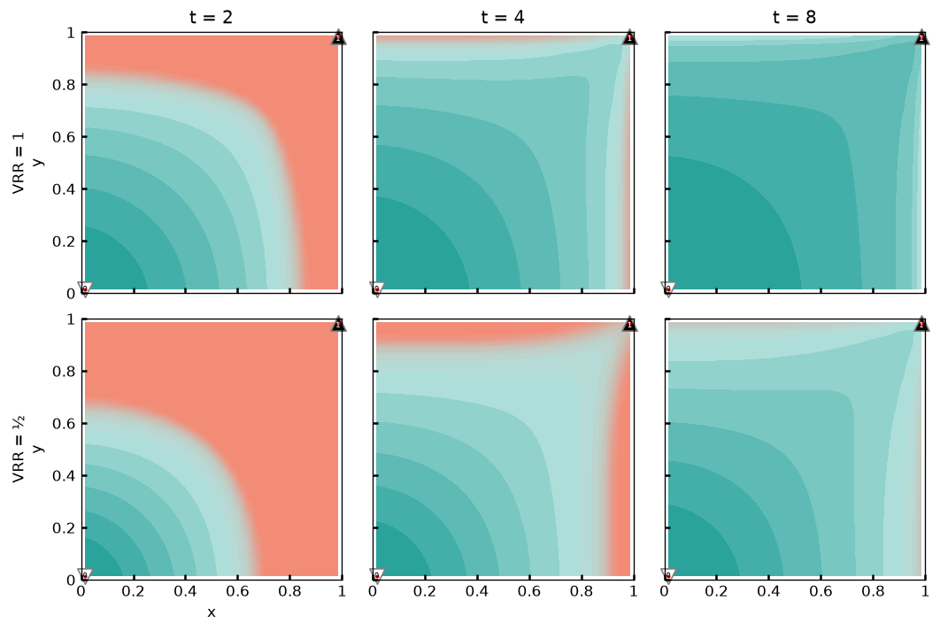
- "saturation": the VRR = ½ row lags from the outset (only half the water has gone in), and by t = 8 it has still not swept the NE corner, whereas VRR = 1 has (mean saturation 0.79, against 0.89). Note also the shape: compared at equal injected volume (VRR = 1 at t = 4 against VRR = ½ at t = 8, both one pore volume) the two sweeps are close, but not equal -- an rms difference of 0.06 in saturation.
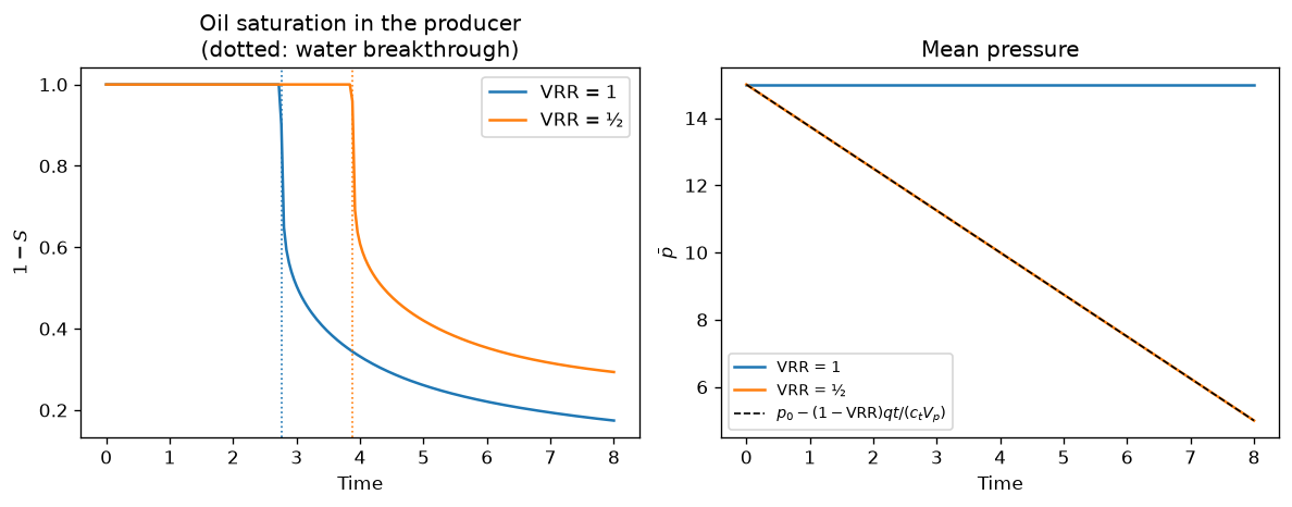
- "histories" (left): breakthrough (dotted) is deferred from t = 2.8 to t = 3.9. Measured in injected volume, though, it arrives sooner: after 0.49 pore volumes, against 0.69. Under-injecting buys time, but sweeps less efficiently, the expansion drive adding a drift towards the producer.
- "histories" (right): the price. $\bar{p}$ falls from 15 to 5, along the material-balance line (dashed), while VRR = 1 holds it at 15.
  1"""Waterflooding while *under*-injecting -- and what it does to the front.
  2
  3The "voidage replacement ratio" (VRR) is the injected volume divided by the
  4produced one. The incompressible model can only ever run `VRR = 1`
  5(`time_stepper` asserts it). With `ct > 0` we may inject less than we produce,
  6the difference being made up by expansion (storage), i.e. by declining pressure.
  7
  8Here the same producer rate is run at `VRR = 1` and at `VRR = ½`, showing that
  9compressibility affects the *saturation* history, not just the pressure:
 10
 11- The front advances more slowly, delaying water breakthrough.
 12- Some of the oil is instead driven by expansion, from all directions, so the
 13  sweep is not simply a "slowed down" version of `VRR = 1`: per unit of water
 14  injected, it is also *less efficient*.
 15- The pressure declines at the rate given by material balance
 16  (see `examples.depletion`), which is the price paid for the deferral.
 17
 18Both the pressure and the transport equation carry their $O(c_t)$ terms
 19(ref `ResSim.ct`), so the saturations stay bounded and, at `VRR = 1`, converge
 20to the incompressible solution as $c_t → 0$ -- verified below.
 21
 22.. warning:: This example is deliberately extreme.
 23
 24    It produces two pore volumes while injecting one,
 25    so the fluids are asked to expand by 100%, i.e.
 26    $ c_t Δ\\bar{p} = 1 $, rather than the $ \\ll 1 $ that "slightly
 27    compressible" implies. The behaviour below is self-consistent and
 28    qualitatively right, but not quantitatively trustworthy. NB: lowering `ct`
 29    does *not* remedy it, the voidage being what sets the demanded expansion
 30    (ref the "Compressibility" section of the docs).
 31
 32In the figures:
 33
 34- "saturation": the VRR = ½ row lags from the outset (only half the water has
 35  gone in), and by t = 8 it has still not swept the NE corner, whereas VRR = 1
 36  has (mean saturation 0.79, against 0.89). Note also the *shape*: compared at
 37  equal injected volume (VRR = 1 at t = 4 against VRR = ½ at t = 8, both one
 38  pore volume) the two sweeps are close, but not equal -- an rms difference of
 39  0.06 in saturation.
 40- "histories" (left): breakthrough (dotted) is deferred from t = 2.8 to t = 3.9.
 41  Measured in injected volume, though, it arrives *sooner*: after 0.49 pore
 42  volumes, against 0.69. Under-injecting buys time, but sweeps less
 43  efficiently, the expansion drive adding a drift towards the producer.
 44- "histories" (right): the price. $\\bar{p}$ falls from 15 to 5, along the
 45  material-balance line (dashed), while VRR = 1 holds it at 15.
 46"""
 47
 48from mpl_tools.place import freshfig
 49import numpy as np
 50
 51from TPFA_ResSim import ResSim
 52from TPFA_ResSim.plotting import show
 53
 54## Setup
 55q = .25
 56ct = .1
 57dt = .04
 58nSteps = 200
 59tt = dt*np.arange(nSteps + 1)
 60oil_only = np.zeros(32*32)
 61
 62
 63def waterflood(vrr, ct=ct, P0=15.):
 64    """Produce at rate `q`, inject at `vrr*q`."""
 65    model = ResSim(Lx=1, Ly=1, Nx=32, Ny=32, ct=ct,
 66                   wells=[dict(xy=[0, 0], rate=+vrr*q),
 67                          dict(xy=[1, 1], rate=-q)])
 68    kwargs: dict = dict(P0=P0*np.ones(model.Nxy)) if ct else {}
 69    return (model,) + model.sim(dt, nSteps, oil_only, pbar=False, **kwargs)
 70
 71
 72## Simulate
 73model, SS_full, PP_full = waterflood(vrr=1)
 74_    , SS_half, PP_half = waterflood(vrr=.5)
 75# At VRR = 1 there is no net voidage, so the incompressible model is the
 76# `ct → 0` limit. Check that the deviation from it is indeed O(ct), i.e. that
 77# dividing `ct` by ten divides the deviation by (about) ten.
 78_, SS_inc , _ = waterflood(vrr=1, ct=0)
 79_, SS_lowc, _ = waterflood(vrr=1, ct=ct/10)
 80dev = [abs(S - SS_inc).max() for S in [SS_full, SS_lowc]]
 81assert 8 < dev[0]/dev[1] < 12, dev
 82
 83iprd = model.xy2ind(*model.wells.xy[1])
 84breakthrough = [dt*np.argmax(S[:, iprd] > .01) for S in [SS_full, SS_half]]
 85
 86## Plot: the front, at equal times
 87fig, axs = freshfig("Voidage replacement -- saturation", nrows=2, ncols=3,
 88                    sharex=True, sharey=True, figsize=(9, 6))
 89for row, (SS, vrr) in enumerate(zip([SS_full, SS_half], ["1", "½"])):
 90    for col, t in enumerate([2, 4, 8]):
 91        model.plt_field(axs[row, col], SS[int(t/dt)], "oil", wells=dict(size=.4),
 92                        colorbar=False, finalize=False, labels=False,
 93                        title=(f"t = {t}" if row == 0 else ""))
 94    axs[row, 0].set_ylabel(f"VRR = {vrr}\ny")
 95axs[1, 0].set_xlabel("x")
 96fig.tight_layout()
 97
 98## Plot: breakthrough, and the pressure paid for it
 99fig, (ax1, ax2) = freshfig("Voidage replacement -- histories",
100                           ncols=2, figsize=(10, 4))
101
102for SS, vrr, t_bt in zip([SS_full, SS_half], ["1", "½"], breakthrough):
103    h, = ax1.plot(tt, 1 - SS[:, iprd], label=f"VRR = {vrr}")
104    ax1.axvline(t_bt, c=h.get_color(), ls=":", lw=1)
105ax1.set(title="Oil saturation in the producer\n(dotted: water breakthrough)",
106        xlabel="Time", ylabel="$1 - S$")
107ax1.legend()
108
109for PP, vrr in zip([PP_full, PP_half], ["1", "½"]):
110    ax2.plot(tt, PP.mean(axis=1), label=f"VRR = {vrr}")
111ax2.plot(tt, 15 - .5*q*tt/(ct*model.h2*model.por.sum()), "k--", lw=1,
112         label="$p_0 - (1 - \\mathrm{VRR}) q t / (c_t V_p)$")
113ax2.set(title="Mean pressure", xlabel="Time", ylabel="$\\bar{p}$")
114ax2.legend(fontsize="small")
115fig.tight_layout()
116
117# Under-injecting defers breakthrough, but not for free:
118assert breakthrough[1] > breakthrough[0]
119assert PP_half[-1].mean() < PP_full[-1].mean()
120
121# Regression values, checked by `tests/test_examples.py`.
122__digest__ = dict(sat_full = SS_full[-1],
123                  sat_half = SS_half[-1],
124                  prd_full = SS_full[:, iprd],
125                  prd_half = SS_half[:, iprd],
126                  p_half   = PP_half.mean(axis=1))
127
128if __name__ == "__main__":
129    show()