examples.well_path
Well paths: a well completed in many cells rather than one.
well_path walks a polyline through the grid and returns the cells it
traverses, their well indices (peaceman_WI, scaled by how much of each
cell is actually traversed), and w, the resulting split of the well's rate.
Several completions then act as a single well simply by being several wells:
ResSim.assemble_wells superimposes them.
Here a point injector in the SW corner is replaced by a "horizontal" one along the whole west edge, at the same total rate, and the difference in sweep is the point of the exercise.
The rate split, though, is a choice, and the two modes of control make it differently:
- under rate control,
wapportions the rate in proportion to the well index -- a static allocation, exact only if the completions see equal pressure; - under BHP control, they instead share a single $ p_\mathrm{bh} $, and each flows whatever its own drawdown implies -- so the allocation is solved for, and follows the pressure field as it evolves.
This is incompressible (ct = 0), so the BHP-controlled path must still inject
exactly what the producer takes -- it only gets to choose where along itself.
Note also that a BHP well anchors the otherwise pure-Neumann pressure equation.
In the figures:
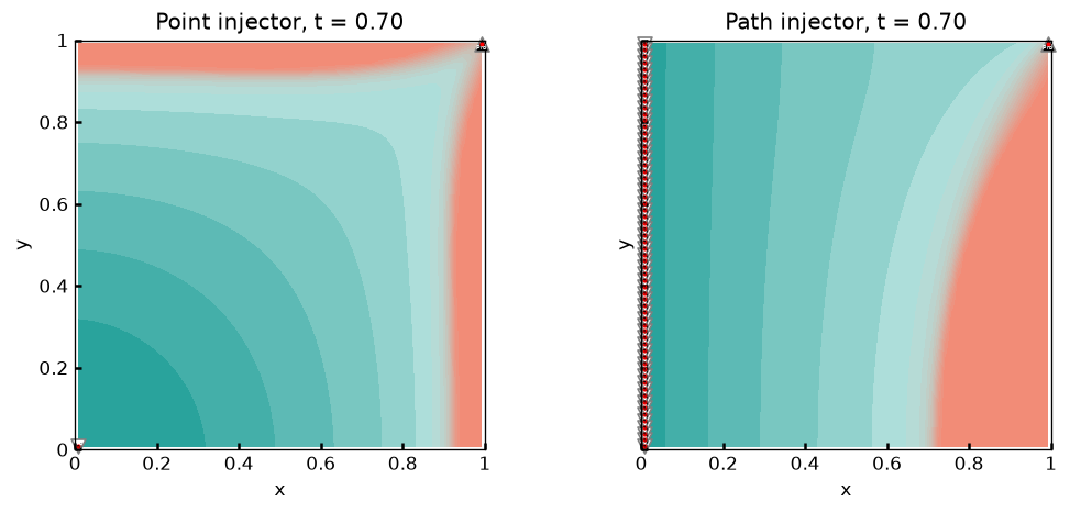
- "sweep": the point injector drives one front out of the corner, symmetric about the diagonal (the mean saturation is 0.66 in both the NW and the SE quadrant). The path drives a broad one off the whole west edge, and thereby breaks that symmetry: it floods the NW hard (0.87) at the expense of the SE (0.33), and in fact sweeps less of the field overall (83% against 90% of cells contacted). Longer is not automatically better -- which is the sort of thing one drills a path to find out. The well markers trace the path.
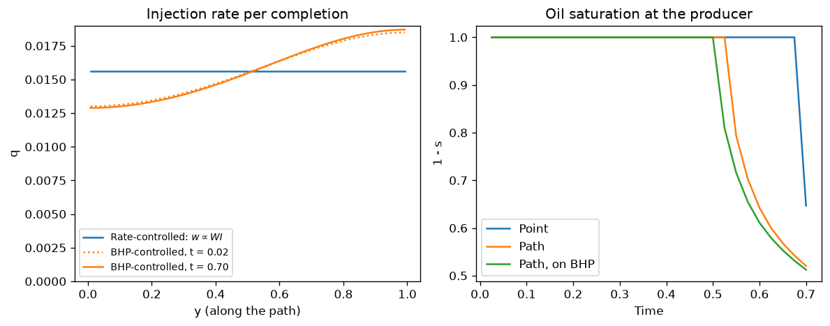
- "allocation" (left): the static split
wis uniform here, this path crossing each cell of the west column fully -- it knows only the geometry. The BHP-solved split is not: the toe of the well, being nearer the producer, takes some 45% more than the heel. That ratio is set mostly by the geometry too, and so barely drifts as the flood develops. - "allocation" (right): oil saturation at the producer. The path breaks through at step 21, against the point injector's 27, and its water cut then climbs faster -- the near half of the reservoir having been flooded preferentially.
  1"""Well *paths*: a well completed in many cells rather than one.
  2
  3`well_path` walks a polyline through the grid and returns the cells it
  4traverses, their well indices (`peaceman_WI`, scaled by how much of each
  5cell is actually traversed), and `w`, the resulting split of the well's rate.
  6Several completions then act as a single well simply by *being* several wells:
  7`ResSim.assemble_wells` superimposes them.
  8
  9Here a point injector in the SW corner is replaced by a "horizontal" one along
 10the whole west edge, at the same total rate, and the difference in sweep is the
 11point of the exercise.
 12
 13The rate split, though, is a choice, and the two modes of control make it
 14differently:
 15
 16- under **rate** control, `w` apportions the rate in proportion to the well
 17  index -- a static allocation, exact only if the completions see equal
 18  pressure;
 19- under **BHP** control, they instead share a single $ p_\\mathrm{bh} $, and each
 20  flows whatever its own drawdown implies -- so the allocation is *solved for*,
 21  and follows the pressure field as it evolves.
 22
 23This is incompressible (`ct = 0`), so the BHP-controlled path must still inject
 24exactly what the producer takes -- it only gets to choose *where* along itself.
 25Note also that a BHP well anchors the otherwise pure-Neumann pressure equation.
 26
 27In the figures:
 28
 29- "sweep": the point injector drives one front out of the corner, symmetric
 30  about the diagonal (the mean saturation is 0.66 in *both* the NW and the SE
 31  quadrant). The path drives a broad one off the whole west edge, and thereby
 32  breaks that symmetry: it floods the NW hard (0.87) at the expense of the SE
 33  (0.33), and in fact sweeps *less* of the field overall (83% against 90% of
 34  cells contacted). Longer is not automatically better -- which is the sort of
 35  thing one drills a path to find out. The well markers trace the path.
 36- "allocation" (left): the static split `w` is uniform here, this path crossing
 37  each cell of the west column fully -- it knows only the geometry. The
 38  BHP-solved split is not: the toe of the well, being nearer the producer, takes
 39  some 45% more than the heel. That ratio is set mostly by the geometry too, and
 40  so barely drifts as the flood develops.
 41- "allocation" (right): oil saturation at the producer. The path breaks through
 42  at step 21, against the point injector's 27, and its water cut then climbs
 43  faster -- the near half of the reservoir having been flooded preferentially.
 44"""
 45
 46from mpl_tools.place import freshfig
 47import numpy as np
 48
 49from TPFA_ResSim import ResSim, well_path
 50from TPFA_ResSim.plotting import show
 51
 52## Setup
 53rw = 1e-3
 54nSteps = 28
 55dt = .7/nSteps
 56tt = dt*(1 + np.arange(nSteps))
 57
 58def waterflood(injector):
 59    """A unit square, producing from the NE corner at a rate of 1.
 60
 61    The `injector` is a well record; ref `ResSim.wells`, which is also what
 62    turns its `path` into completions -- there being nothing further to do.
 63    """
 64    model = ResSim(Lx=1, Ly=1, Nx=64, Ny=64,
 65                   wells=[injector, dict(name="Prd", xy=[1, 1], rate=-1)])
 66    SS, PP = model.sim(dt, nSteps, model.swc*np.ones(model.Nxy), pbar=False)
 67    return model, SS
 68
 69# The path, and its discretization into completions
 70proto = ResSim(Lx=1, Ly=1, Nx=64, Ny=64)
 71xy, WI, w = well_path(proto, [[0, 0], [0, 1]], rw)
 72assert len(xy) == proto.Ny, "The west edge is one cell wide, and Ny cells long."
 73
 74## Simulate: a point injector, the same as a path, and the path on BHP.
 75point, SS_point = waterflood(dict(name="Inj", xy=[0, 0], rate=1))
 76path , SS_path  = waterflood(dict(name="Inj", path=[[0, 0], [0, 1]], rate=1, rw=rw))
 77onbhp, SS_onbhp = waterflood(dict(name="Inj", path=[[0, 0], [0, 1]], bhp=3., rw=rw))
 78
 79# The completions of the injector, as grouped by `wells`
 80inj = path.wells.group == 0
 81assert inj.sum() == len(xy) and np.allclose(path.wells.WI[inj], WI)
 82
 83# Incompressible => whatever the control, the injection must match the production
 84for model in [path, onbhp]:
 85    assert np.allclose(model.wells.actual_rates[inj].sum(axis=0), 1)
 86    assert np.allclose(model.wells.rates_by_well, [[1], [-1]])   # (nWell, nSteps)
 87
 88## Plot: the resulting sweeps
 89fig, axs = freshfig("Well path -- sweep", ncols=2, sharex=True, sharey=True,
 90                    figsize=(9, 4))
 91for ax, (name, model, SS) in zip(axs, [("Point injector", point, SS_point),
 92                                       ("Path injector", path, SS_path)]):
 93    model.plt_field(ax, SS[-1], "oil", finalize=False, colorbar=False,
 94                    title=f"{name}, t = {dt*nSteps:.2f}", wells=dict(size=.3))
 95fig.tight_layout()
 96
 97## Plot: how the rate gets allocated along the path, and what is produced
 98fig, (ax1, ax2) = freshfig("Well path -- allocation", ncols=2, figsize=(10, 4))
 99
100yy = xy[:, 1]
101ax1.plot(yy, path.wells.actual_rates[inj, -1], label="Rate-controlled: $w \\propto WI$")
102for k, ls in [(0, ":"), (nSteps - 1, "-")]:
103    ax1.plot(yy, onbhp.wells.actual_rates[inj, k], ls, c="C1",
104             label=f"BHP-controlled, t = {tt[k]:.2f}")
105ax1.set(title="Injection rate per completion", xlabel="y (along the path)",
106        ylabel="q", ylim=0)
107ax1.legend(fontsize="small")
108
109prd = [point.xy2ind(*point.wells.xy[-1])]
110for name, SS in [("Point", SS_point), ("Path", SS_path), ("Path, on BHP", SS_onbhp)]:
111    ax2.plot(tt, 1 - SS[1:, prd[0]], label=name)
112ax2.set(title="Oil saturation at the producer", xlabel="Time", ylabel="1 - s")
113ax2.legend()
114fig.tight_layout()
115
116# Regression values, checked by `tests/test_examples.py`.
117__digest__ = dict(alloc_static = w,
118                  alloc_bhp    = onbhp.wells.actual_rates[inj, -1],
119                  sat_point    = SS_point[-1, ::600],
120                  sat_path     = SS_path[-1, ::600])
121
122if __name__ == "__main__":
123    show()