examples.pressure_diffusion
Finite-speed pressure propagation, and the pressure "gauge".
With ct = 0 the pressure equation is elliptic: the whole field re-adjusts
instantaneously whenever a rate changes, and (since the boundaries are closed)
the solution is only determined up to an additive constant.
With ct > 0 it is parabolic -- a diffusion equation with diffusivity
$$ η = K λ / (φ c_t) $$
so a rate change is felt only after a delay of the order $ r^2/η $ at distance $r$.
The elliptic solution is recovered as $ t → ∞ $ (or $ c_t → 0 $), as shown below.
Moreover, the pressure level is now pinned by the initial condition P0
(the model keeps track of absolute pressure, not just its gradients).
Notes on the setup:
- The reservoir is initialised fully water-saturated, so that the total mobility
$λ = 1$ is uniform and constant, isolating the pressure physics
(i.e. $η = 100$ everywhere, since
K = por = 1andct = .01). It stays that way exactly: $s = 1$ is a fixed point of the transport step (refResSim.storage_rate), whatever the wells do. Asserted below. - The rates are balanced (as they must be for the
ct = 0comparison run), whence the storage terms cancel and the mean pressure stays atP0exactly. This conveniently fixes the (otherwise arbitrary) level of the elliptic solution: we centre it on its own mean.
In the figures:
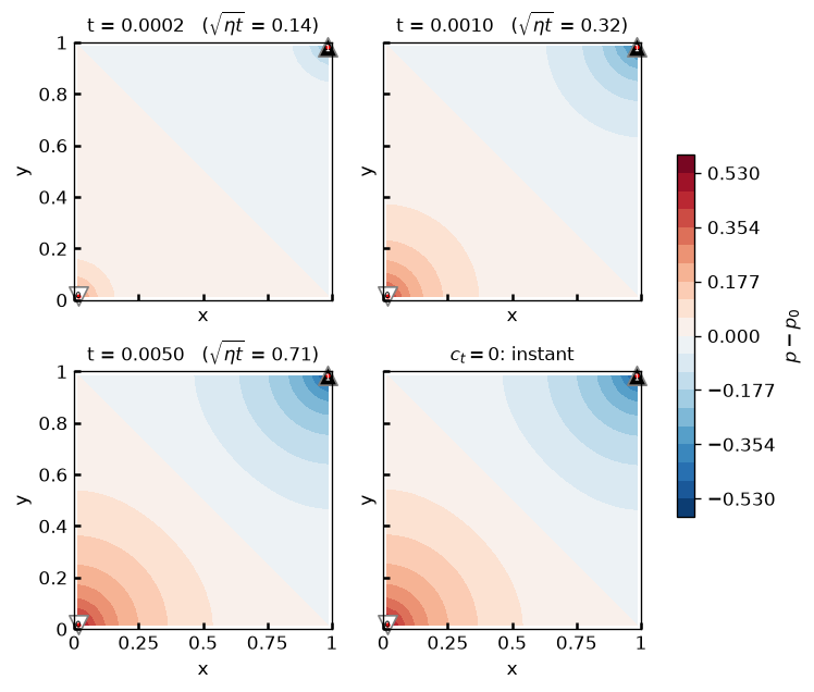
- "Pressure diffusion": at t = 0.0002 only the immediate surroundings of the
two wells have responded -- the middle of the domain is still at
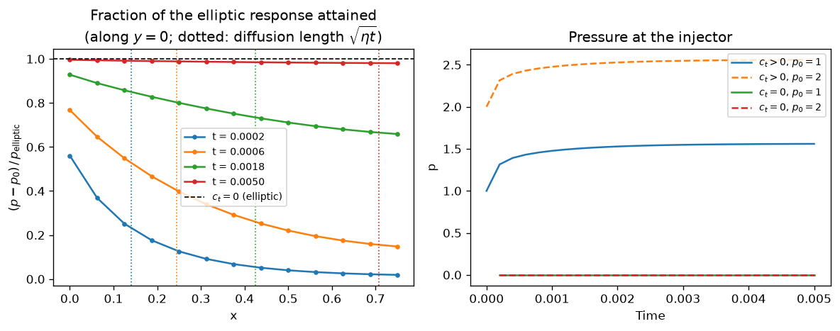
P0(white) -- while by t = 0.005 the field is barely distinguishable from the elliptic one (bottom right). The four panels share their colour scale. - "profiles & gauge" (left): the same, quantified along the y = 0 edge. At the earliest time, the far half of that line has attained under 2% of its eventual (elliptic) response; at the latest time, some 98%. The dotted verticals mark the diffusion length $\sqrt{ηt}$: an indication of scale, not a sharp front.
- "profiles & gauge" (right): the two
ct > 0curves are separated by exactly the difference of theirP0(asserted below) -- the absolute level is meaningful, and remembered. The twoct = 0curves instead coincide, at 0:P0is ignored, and the level is merely that of the grounded cell.
  1"""Finite-speed pressure propagation, and the pressure "gauge".
  2
  3With `ct = 0` the pressure equation is *elliptic*: the whole field re-adjusts
  4**instantaneously** whenever a rate changes, and (since the boundaries are closed)
  5the solution is only determined up to an additive constant.
  6
  7With `ct > 0` it is *parabolic* -- a diffusion equation with diffusivity
  8
  9$$ η = K λ / (φ c_t) $$
 10
 11so a rate change is felt only after a delay of the order $ r^2/η $ at distance $r$.
 12The elliptic solution is recovered as $ t → ∞ $ (or $ c_t → 0 $), as shown below.
 13Moreover, the pressure level is now pinned by the initial condition `P0`
 14(the model keeps track of *absolute* pressure, not just its gradients).
 15
 16Notes on the setup:
 17
 18- The reservoir is initialised **fully water-saturated**, so that the total mobility
 19  $λ = 1$ is uniform and constant, isolating the pressure physics
 20  (i.e. $η = 100$ everywhere, since `K = por = 1` and `ct = .01`).
 21  It stays that way *exactly*: $s = 1$ is a fixed point of the transport step
 22  (ref `ResSim.storage_rate`), whatever the wells do. Asserted below.
 23- The rates are balanced (as they must be for the `ct = 0` comparison run),
 24  whence the storage terms cancel and the *mean* pressure stays at `P0` exactly.
 25  This conveniently fixes the (otherwise arbitrary) level of the elliptic solution:
 26  we centre it on its own mean.
 27
 28In the figures:
 29
 30- "Pressure diffusion": at t = 0.0002 only the immediate surroundings of the
 31  two wells have responded -- the middle of the domain is still at `P0` (white)
 32  -- while by t = 0.005 the field is barely distinguishable from the elliptic
 33  one (bottom right). The four panels share their colour scale.
 34- "profiles & gauge" (left): the same, quantified along the y = 0 edge. At the
 35  earliest time, the far half of that line has attained under 2% of its
 36  eventual (elliptic) response; at the latest time, some 98%. The dotted
 37  verticals mark the diffusion length $\\sqrt{ηt}$: an indication of scale,
 38  not a sharp front.
 39- "profiles & gauge" (right): the two `ct > 0` curves are separated by exactly
 40  the difference of their `P0` (asserted below) -- the absolute level is
 41  meaningful, and remembered. The two `ct = 0` curves instead coincide, at 0:
 42  `P0` is ignored, and the level is merely that of the grounded cell.
 43"""
 44
 45from mpl_tools.place import freshfig
 46import numpy as np
 47
 48from TPFA_ResSim import ResSim
 49from TPFA_ResSim.plotting import show
 50
 51## Setup
 52wells = [dict(xy=[0, 0], rate=+.25), dict(xy=[1, 1], rate=-.25)]
 53grid: dict = dict(Lx=1, Ly=1, Nx=32, Ny=32)
 54
 55model = ResSim(**grid, wells=wells, ct=.01)
 56model_inc = ResSim(**grid, wells=wells)  # ct = 0
 57
 58eta = 1/model.ct  # Diffusivity (since K = por = λ = 1)
 59dt = 2e-4
 60nSteps = 25
 61water_sat0 = np.ones(model.Nxy)
 62P0 = np.ones(model.Nxy)
 63
 64## Simulate
 65SS, PP = model.sim(dt, nSteps, water_sat0, P0=P0, pbar=False)
 66assert (SS == 1).all(), "The reservoir should remain fully water-saturated."
 67_, PP_inc = model_inc.sim(dt, nSteps, water_sat0, pbar=False)
 68# Same, but starting from a higher pressure level
 69_, PP_hi = model.sim(dt, nSteps, water_sat0, P0=P0 + 1, pbar=False)
 70_, PP_inc_hi = model_inc.sim(dt, nSteps, water_sat0, P0=P0 + 1, pbar=False)
 71
 72# The elliptic solution is the same at all times here (mobility is constant).
 73# Its level is arbitrary: centre it, matching the (conserved) mean of `PP`.
 74elliptic = PP_inc[1] - PP_inc[1].mean()
 75
 76## Plot: the pressure disturbance, dp, spreading out
 77snapshots = [1, 5, nSteps]
 78vmax = 1.05*np.abs(elliptic).max()
 79kws: dict = dict(levels=np.linspace(-vmax, vmax, 21), cmap="RdBu_r",
 80                 colorbar=False, finalize=False, wells=dict(size=.4))
 81
 82fig, axs = freshfig("Pressure diffusion", nrows=2, ncols=2,
 83                    sharex=True, sharey=True, figsize=(7, 6))
 84for ax, k in zip(axs.ravel(), snapshots + [None]):
 85    if k is None:
 86        cc = model.plt_field(ax, elliptic, **kws, title="$c_t = 0$: instant")
 87    else:
 88        cc = model.plt_field(ax, PP[k] - P0, **kws,
 89                             title=f"t = {k*dt:.4f}   "
 90                                   f"($\\sqrt{{ηt}}$ = {np.sqrt(eta*k*dt):.2f})")
 91    ax.title.set_fontsize("medium")
 92fig.colorbar(cc, ax=axs, shrink=.6, label="$p - p_0$")
 93
 94## Plot: how much of the eventual response has arrived, and where
 95fig, (ax1, ax2) = freshfig("Pressure diffusion -- profiles & gauge",
 96                           ncols=2, figsize=(10, 4))
 97
 98# Sample along the y=0 edge, stopping short of the (anti-symmetric) corner,
 99# where the elliptic reference vanishes and the ratio below is meaningless.
100xx = np.linspace(0, .75, 13)
101line = [model.xy2ind(x, 0) for x in xx]
102
103for k in [1, 3, 9, nSteps]:
104    h, = ax1.plot(xx, ((PP[k] - P0)/elliptic)[line], "-o", ms=3,
105                  label=f"t = {k*dt:.4f}")
106    # The diffusion length -- an indication of scale, not a sharp front
107    ax1.axvline(np.sqrt(eta*k*dt), c=h.get_color(), ls=":", lw=1)
108ax1.axhline(1, c="k", ls="--", lw=1, label="$c_t = 0$ (elliptic)")
109ax1.set(title="Fraction of the elliptic response attained\n"
110              "(along $y=0$; dotted: diffusion length $\\sqrt{ηt}$)",
111        xlabel="x", ylabel="$(p - p_0) \\, / \\, p_\\mathrm{elliptic}$")
112ax1.legend(fontsize="small")
113
114# Gauge: is the absolute pressure level meaningful?
115tt = dt*np.arange(nSteps + 1)
116iw = model.xy2ind(*model.wells.xy[0])
117ax2.plot(tt, PP[:, iw]   , "-" , c="C0", label="$c_t>0$, $p_0=1$")
118ax2.plot(tt, PP_hi[:, iw], "--", c="C1", label="$c_t>0$, $p_0=2$")
119ax2.plot(tt[1:], PP_inc[1:, iw]   , "-" , c="C2", label="$c_t=0$, $p_0=1$")
120ax2.plot(tt[1:], PP_inc_hi[1:, iw], "--", c="C3", label="$c_t=0$, $p_0=2$")
121ax2.set(title="Pressure at the injector", xlabel="Time", ylabel="p")
122ax2.legend(fontsize="small")
123fig.tight_layout()
124
125# With ct > 0 the two curves are offset by exactly the offset in `P0`:
126assert np.allclose(PP_hi - PP, 1)
127# With ct = 0, `P0` is simply ignored, and the level is that of the "grounding"
128# of cell 0 (ref article p. 13). Indeed, summing all rows of that (modified)
129# system leaves `2 K p[0] = sum(Q) = 0`, i.e. it pins the pressure of cell (0,0):
130assert np.allclose(PP_inc[1:], PP_inc_hi[1:])
131assert np.allclose(PP_inc[1:, 0], 0)
132
133# Regression values, checked by `tests/test_examples.py`.
134__digest__ = dict(dp_early = PP[1] - P0,
135                  dp_late  = PP[nSteps] - P0,
136                  elliptic = elliptic,
137                  p_inj    = PP[:, iw])
138
139if __name__ == "__main__":
140    show()