examples.well_control
Rate control, BHP control, and the well model that connects them.
A well can be told what to do in two ways: give it a rate (rate, ref
Wells.rates; negative to produce) and let its pressure follow, or give it a
pressure (bhp, ref Wells.bhp) and let its rate follow -- as ResSim.wells
accepts either. Both need a well model -- the well index (peaceman_WI,
whence the rw of the record) -- because a well is far smaller than the cell
that holds it, so its cell pressure is not its wellbore pressure.
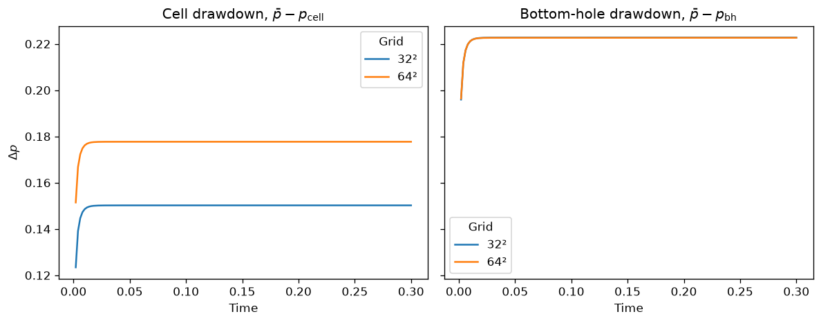
That distinction is the first thing shown here: the cell pressure is a grid artefact, whereas the bottom-hole pressure obtained from it is not.
The two modes are then contrasted on the same closed, depleting reservoir
(cf. examples.depletion), where they behave quite differently:
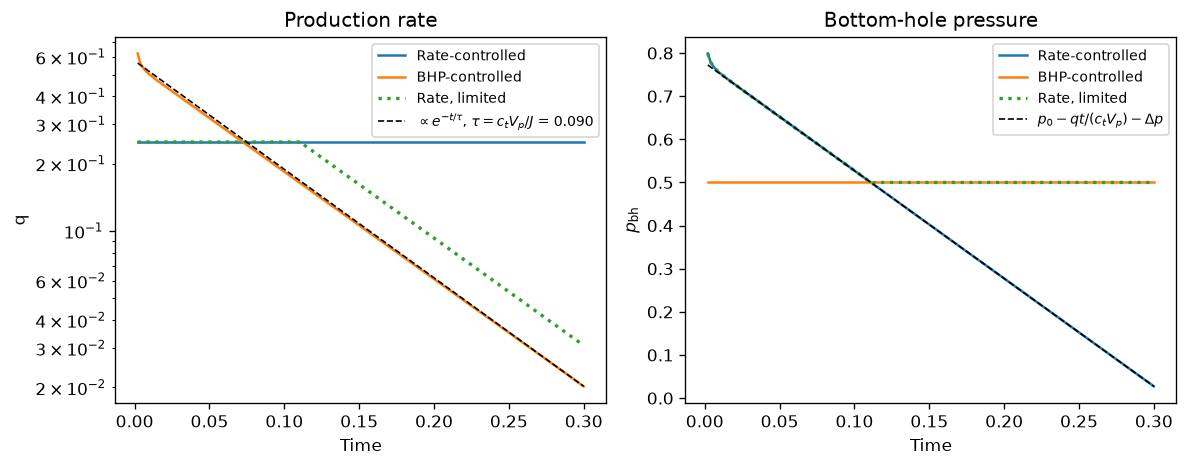
- at constant rate, the pressure declines linearly, as material balance dictates: $ d\bar{p}/dt = -q / (c_t V_p) $;
- at constant BHP, the rate declines exponentially, $ q ∝ e^{-t/τ} $ with $ τ = c_t V_p / J $, since combining that same material balance with the well model, $ q = J (\bar{p} - p_\mathrm{bh}) $, gives a linear ODE. (The productivity index $ J $ differs from $ WI λ_t $ by the geometry between the well and the average pressure.)
Neither mode alone is how a well is actually run: the industry standard is a
rate target with a BHP limit, i.e. whichever of the two currently binds.
The model does not switch modes natively, but ResSim.well_controls returns
both controls, so an override can switch between them -- lagged by the step
whose pressure it must judge from. That is the third case shown here.
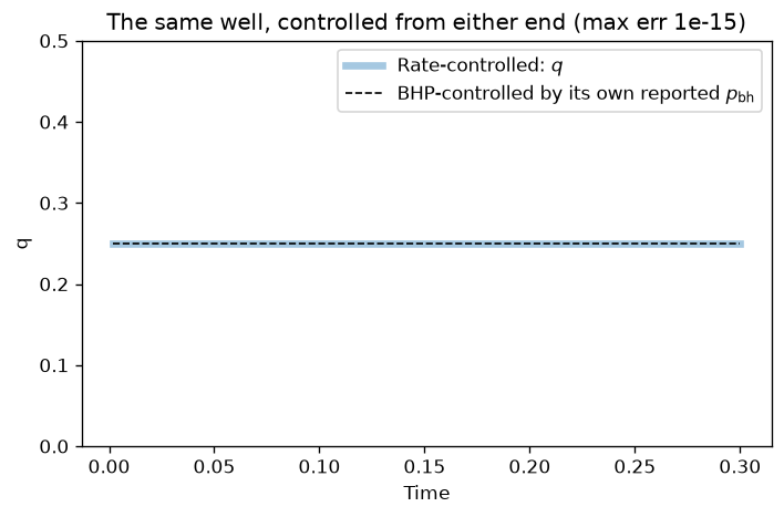
Finally, the two are shown to be one and the same model, seen from either end: prescribing the BHP that the rate-controlled run reported recovers that run exactly (to ~1e-15).
In the figures:
- "diagnostic": refining 32² → 64² moves the producer's cell pressure by a lot (left), while the bottom-hole pressure inferred from it barely moves (right). Only the latter is a property of the well.
- "modes" (left): the rate is flat by construction under rate control, and decays under BHP control -- as a straight line on the log axis, i.e. exponentially, with the analytic slope (dashed). The rate-with-a-limit case traces the former until the limit binds, and joins the latter thereafter (above it, having drained less by then, hence at a higher pressure).
- "modes" (right): the mirror image. The BHP falls linearly under rate control (material balance), and is flat by construction under BHP control -- while the limited well does both in turn, its corner marking the switch.
- "duality": feeding the left run's BHP back in as the control reproduces its rate to machine precision.
  1"""Rate control, BHP control, and the well model that connects them.
  2
  3A well can be told *what to do* in two ways: give it a rate (`rate`, ref
  4`Wells.rates`; negative to produce) and let its pressure follow, or give it a
  5pressure (`bhp`, ref `Wells.bhp`) and let its rate follow -- as `ResSim.wells`
  6accepts either. Both need a **well model** -- the well index (`peaceman_WI`,
  7whence the `rw` of the record) -- because a well is far smaller than the cell
  8that holds it, so its cell pressure is not its wellbore pressure.
  9
 10That distinction is the first thing shown here: the cell pressure is a *grid
 11artefact*, whereas the bottom-hole pressure obtained from it is not.
 12
 13The two modes are then contrasted on the same closed, depleting reservoir
 14(cf. `examples.depletion`), where they behave quite differently:
 15
 16- at constant **rate**, the pressure declines linearly, as material balance
 17  dictates: $ d\\bar{p}/dt = -q / (c_t V_p) $;
 18- at constant **BHP**, the rate declines *exponentially*,
 19  $ q ∝ e^{-t/τ} $ with $ τ = c_t V_p / J $, since combining that same material
 20  balance with the well model, $ q = J (\\bar{p} - p_\\mathrm{bh}) $, gives a
 21  linear ODE. (The productivity index $ J $ differs from $ WI λ_t $ by the
 22  geometry between the well and the average pressure.)
 23
 24Neither mode alone is how a well is actually run: the industry standard is a
 25rate *target* with a BHP *limit*, i.e. whichever of the two currently binds.
 26The model does not switch modes natively, but `ResSim.well_controls` returns
 27both controls, so an override can switch between them -- lagged by the step
 28whose pressure it must judge from. That is the third case shown here.
 29
 30Finally, the two are shown to be one and the same model, seen from either end:
 31prescribing the BHP that the rate-controlled run *reported* recovers that run
 32exactly (to ~1e-15).
 33
 34In the figures:
 35
 36- "diagnostic": refining 32² → 64² moves the producer's cell pressure by a lot
 37  (left), while the bottom-hole pressure inferred from it barely moves (right).
 38  Only the latter is a property of the *well*.
 39- "modes" (left): the rate is flat by construction under rate control, and
 40  decays under BHP control -- as a straight line on the log axis, i.e.
 41  exponentially, with the analytic slope (dashed). The rate-with-a-limit case
 42  traces the former until the limit binds, and joins the latter thereafter
 43  (above it, having drained less by then, hence at a higher pressure).
 44- "modes" (right): the mirror image. The BHP falls linearly under rate control
 45  (material balance), and is flat by construction under BHP control -- while the
 46  limited well does both in turn, its corner marking the switch.
 47- "duality": feeding the left run's BHP back in as the control reproduces its
 48  rate to machine precision.
 49"""
 50
 51from mpl_tools.place import freshfig
 52import numpy as np
 53
 54from TPFA_ResSim import ResSim
 55from TPFA_ResSim.plotting import show
 56
 57## Setup
 58q = .25          # the rate-controlled rate
 59p_bh = .5        # the BHP-controlled pressure
 60rw = 1e-3        # well radius
 61ct = .1
 62dt, nSteps = 2e-3, 150
 63tt = dt*np.arange(1, nSteps + 1)
 64
 65def depleter(N=32, cls=ResSim, **control):
 66    """A single producer at the centre of a closed square. Cf. `examples.depletion`.
 67
 68    The `control` is a `rate` and/or a `bhp`; `rw` is what gives it a well model.
 69    """
 70    return cls(Lx=1, Ly=1, Nx=N, Ny=N, ct=ct,
 71               wells=[dict(xy=[.5, .5], rw=rw, **control)])
 72
 73class Limited(ResSim):
 74    """Rate control with a BHP limit, by overriding `ResSim.well_controls`.
 75
 76    The rate target is held for as long as it can be delivered without drawing
 77    the well below `p_bh`; thereafter the well switches to BHP control at it.
 78    The switch is judged from the *previous* step's pressure, since the new one
 79    is not yet known (indeed it depends on the choice) -- so the limit is
 80    breached for the one step in which it comes to bind.
 81    """
 82
 83    def well_controls(self, S, P, k):
 84        ctrl = super().well_controls(S, P, k)
 85        if P is None:
 86            return ctrl                                # nothing to switch on
 87        would = self.bhp(S, P, ctrl["rates"])          # if rate-controlled
 88        ctrl["bhp"] = np.where(would < p_bh, p_bh, np.nan)
 89        return ctrl
 90
 91def run(model):
 92    SS, PP = model.sim(dt, nSteps, np.zeros(model.Nxy),
 93                       P0=np.ones(model.Nxy), pbar=False)
 94    assert SS.max() == 0, "No water is injected, so none should appear."
 95    return PP
 96
 97## Plot: the diagnostic -- cell pressure is a grid artefact, bottom-hole is not
 98fig, (ax1, ax2) = freshfig("Well control -- diagnostic", ncols=2, figsize=(10, 4),
 99                           sharey=True)
100for N in [32, 64]:
101    model = depleter(N, rate=-q)
102    PP = run(model)
103    pbar = PP.mean(axis=1)
104    ax1.plot(tt, (pbar[1:] - PP[1:, model.xy2ind(*model.wells.xy[0])]), label=f"{N}²")
105    ax2.plot(tt, (pbar[1:] - model.wells.actual_bhp[0]), label=f"{N}²")
106ax1.set(title="Cell drawdown, $\\bar{p} - p_\\mathrm{cell}$",
107        xlabel="Time", ylabel="$\\Delta p$")
108ax2.set(title="Bottom-hole drawdown, $\\bar{p} - p_\\mathrm{bh}$", xlabel="Time")
109for ax in (ax1, ax2):
110    ax.legend(title="Grid")
111fig.tight_layout()
112
113## Simulate: the same reservoir, under either mode of control
114by_rate = depleter(rate=-q)
115PP_rate = run(by_rate)
116by_bhp = depleter(bhp=p_bh)              # NB: no `rate` given
117PP_bhp = run(by_bhp)
118limited = depleter(cls=Limited, rate=-q)  # ... rate, but limited by p_bh
119run(limited)                              # (its rate/BHP is the interest)
120
121# Production, i.e. the negated (signed) rates
122prod_rate, prod_bhp, prod_lim = [-m.wells.actual_rates[0]
123                                 for m in [by_rate, by_bhp, limited]]
124
125# Analytic decline: q = J (pbar - p_bh) with material balance ct Vp dpbar/dt = -q
126Vp = by_bhp.h2 * by_bhp.por.sum()
127J = prod_bhp[-1] / (PP_bhp[-1].mean() - p_bh)
128tau = ct*Vp/J
129
130## Plot: rate and BHP, under either mode
131fig, (ax1, ax2) = freshfig("Well control -- modes", ncols=2, figsize=(10, 4))
132
133ax1.plot(tt, prod_rate, label="Rate-controlled")
134ax1.plot(tt, prod_bhp, label="BHP-controlled")
135ax1.plot(tt, prod_lim, ":", lw=2, label="Rate, limited")
136ax1.plot(tt, prod_bhp[-1]*np.exp((tt[-1] - tt)/tau), "k--",
137         lw=1, label=f"$\\propto e^{{-t/\\tau}}$, $\\tau = c_t V_p / J$ = {tau:.3f}")
138ax1.set(title="Production rate", xlabel="Time", ylabel="q", yscale="log")
139ax1.legend(fontsize="small")
140
141ax2.plot(tt, by_rate.wells.actual_bhp[0], label="Rate-controlled")
142ax2.plot(tt, by_bhp .wells.actual_bhp[0], label="BHP-controlled")
143ax2.plot(tt, limited.wells.actual_bhp[0], ":", lw=2, label="Rate, limited")
144ax2.plot(tt, 1 - q*tt/(ct*Vp) - (PP_rate[-1].mean() - by_rate.wells.actual_bhp[0, -1]),
145         "k--", lw=1, label="$p_0 - qt/(c_t V_p) - \\Delta p$")
146ax2.set(title="Bottom-hole pressure", xlabel="Time", ylabel="$p_\\mathrm{bh}$")
147ax2.legend(fontsize="small")
148fig.tight_layout()
149
150## The duality: prescribe the BHP that the rate-controlled run reported
151replay = depleter(bhp=by_rate.wells.actual_bhp[0])
152PP_replay = run(replay)
153err_P = np.abs(PP_replay - PP_rate).max()
154err_q = np.abs(replay.wells.actual_rates + q).max()
155assert err_P < 1e-12 and err_q < 1e-12, "The two controls are not each other's inverse!"
156
157fig, ax = freshfig("Well control -- duality", figsize=(6, 4))
158ax.plot(tt, prod_rate, lw=4, alpha=.4, label="Rate-controlled: $q$")
159ax.plot(tt, -replay.wells.actual_rates[0], "k--", lw=1,
160        label="BHP-controlled by its own reported $p_\\mathrm{bh}$")
161ax.set(title=f"The same well, controlled from either end (max err {err_q:.0e})",
162       xlabel="Time", ylabel="q", ylim=(0, 2*q))
163ax.legend()
164fig.tight_layout()
165
166# Regression values, checked by `tests/test_examples.py`.
167# NB: the production rates are negated, preserving the pre-v0.3 references.
168__digest__ = dict(rate_of_bhp_ctrl = prod_bhp,
169                  bhp_of_rate_ctrl = by_rate.wells.actual_bhp[0],
170                  p_last_bhp_ctrl  = PP_bhp[-1],
171                  rate_of_limited  = prod_lim,
172                  bhp_of_limited   = limited.wells.actual_bhp[0])
173
174if __name__ == "__main__":
175    show()