examples.buildup
Pressure buildup after shut-in -- a "well test". In metric units.
The producer flows for a while, and is then shut in (rate set to 0). The pressure then builds up, asymptotically towards the average pressure, which is now constant since nothing enters or leaves the (closed) reservoir.
Everything here is a consequence of ct > 0:
- Monitor points further from the well respond later (and, after shut-in, keep declining for a while before turning around: they have not yet "heard" that the well was shut).
- The relaxation is gradual, i.e. it has a memory of the flow history -- this is what makes well testing a viable inference method.
For contrast, we also run the incompressible model -- where a shut-in is
felt everywhere immediately, and completely: the pressure (which is then only
defined up to a constant, ref examples.pressure_diffusion) instantly
becomes uniform. NB: since ct = 0 demands balanced rates, that run needs an
active injector, whose rate is switched off at the same time.
As in examples.depletion, no water is present, so S = 0 throughout --
and, likewise, every pressure plotted here is a cell pressure, not a wellbore
one; ref that example's note on the well model.
Units
Unlike the other examples -- which leave the units unspecified (default)
this one is posed in practical metric units: metres, days, bar, mD, cP,
by changing ResSim.cdarcy to $ C = 0.008527 $.
Moreover, a 2 km square of 100 mD rock at 250 bar, produced at 20 m³/day/m, has a pressure diffusivity of
$$ η = C K λ / (φ c_t) ≈ 4.3 \times 10^4 \; \mathrm{m^2/day} \,, $$
so the well feels the boundary, 1 km away, after some $ r^2/η ≈ 23 $ days -- whence the 12-day flow period and 28-day buildup simulated here.
It also lets the run be interpreted the way a real well test is. During radial transient flow the line-source solution gives
$$ p_i - p = \frac{q μ}{4 π C K} \left[ \ln \frac{4 η t}{e^γ r^2} \right] \,, $$
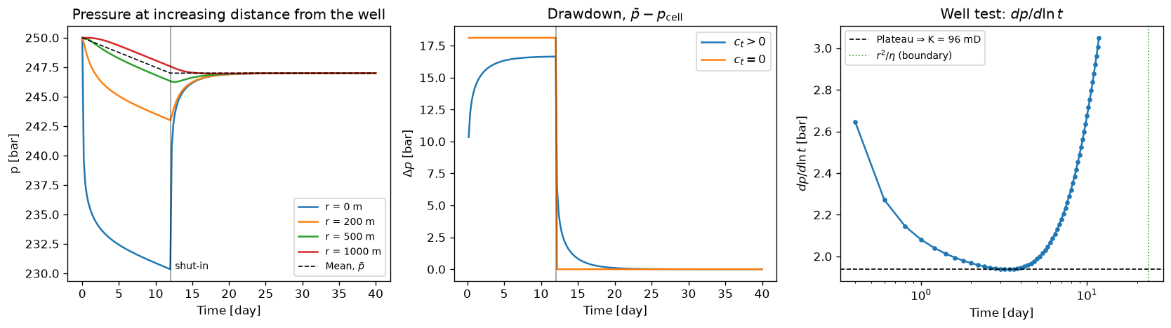
so the semilog derivative $ dp / d\ln t $ plateaus at $ q μ / (4 π C K) $ --
the classic diagnostic of pressure-transient analysis. Being independent of
$ r $, the cell pressure will do (no well model needed), and reading $ K $ off
that plateau recovers the 100 mD that went in, to within 4%. The shortfall is
the time discretization, not the units: at dt = .05 it is 1%.
Nothing here knows that the numbers are metric.
The axis labels below say "[bar]" because this script says so.
cdarcy fixes the arithmetic, not the nomenclature.
In the figures:
- "time series" (left): the delay of the response with distance -- by the time the well (r = 0) has dropped by 12 bar, the r = 1000 m point has barely moved. After the shut-in the near-well pressure recovers at once, whereas the distant points keep declining for a while before turning around: they have not yet heard of it. All then converge on $\bar{p}$ (dashed), now constant.
- "time series" (middle): for
ct > 0the drawdown decays smoothly over the remainder of the run. Forct = 0it is a rectangle: rate on, rate off, and nothing in between. - "time series" (right): the semilog derivative, and the plateau read off its minimum. It is a shallow minimum rather than a flat stretch, being squeezed from both sides: at early times the cell average has not yet resolved the transient, and at late times (dotted) the closed boundary ends the radial regime. Hence the 4%.
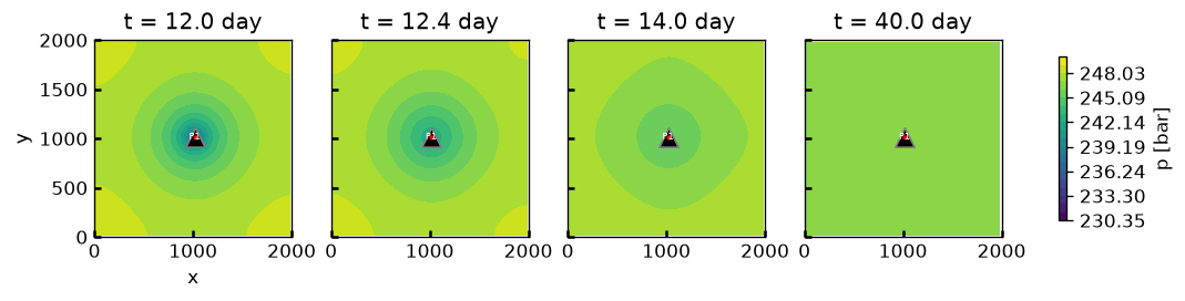
- "pressure": the depression cone filling in -- the sharp, near-well part first, the broad remainder last.
  1"""Pressure buildup after shut-in -- a "well test". **In metric units.**
  2
  3The producer flows for a while, and is then shut in (rate set to 0).
  4The pressure then *builds up*, asymptotically towards the average pressure,
  5which is now constant since nothing enters or leaves the (closed) reservoir.
  6
  7Everything here is a consequence of `ct > 0`:
  8
  9- Monitor points further from the well respond later
 10  (and, after shut-in, keep declining for a while before turning around:
 11  they have not yet "heard" that the well was shut).
 12- The relaxation is gradual, i.e. it has a memory of the flow history --
 13  this is what makes well testing a viable inference method.
 14
 15For contrast, we also run the incompressible model -- where a shut-in is
 16felt everywhere immediately, and completely: the pressure (which is then only
 17defined up to a constant, ref `examples.pressure_diffusion`) instantly
 18becomes uniform. NB: since `ct = 0` demands balanced rates, that run needs an
 19active injector, whose rate is switched off at the same time.
 20
 21As in `examples.depletion`, no water is present, so `S = 0` throughout --
 22and, likewise, every pressure plotted here is a *cell* pressure, not a wellbore
 23one; ref that example's note on the well model.
 24
 25## Units
 26
 27Unlike the other examples -- which leave the units unspecified (default)
 28this one is posed in practical **metric** units: metres, days, bar, mD, cP,
 29by changing `ResSim.cdarcy` to $ C = 0.008527 $.
 30
 31Moreover, a 2 km square of 100 mD rock
 32at 250 bar, produced at 20 m³/day/m, has a pressure diffusivity of
 33
 34$$ η = C K λ / (φ c_t) ≈ 4.3 \\times 10^4 \\; \\mathrm{m^2/day} \\,, $$
 35
 36so the well feels the boundary, 1 km away, after some $ r^2/η ≈ 23 $ days --
 37whence the 12-day flow period and 28-day buildup simulated here.
 38
 39It also lets the run be *interpreted* the way a real well test is. During
 40radial transient flow the line-source solution gives
 41
 42$$ p_i - p = \\frac{q μ}{4 π C K} \\left[ \\ln \\frac{4 η t}{e^γ r^2} \\right] \\,, $$
 43
 44so the semilog derivative $ dp / d\\ln t $ **plateaus** at $ q μ / (4 π C K) $ --
 45the classic diagnostic of pressure-transient analysis. Being independent of
 46$ r $, the *cell* pressure will do (no well model needed), and reading $ K $ off
 47that plateau recovers the 100 mD that went in, to within 4%. The shortfall is
 48the time discretization, not the units: at `dt = .05` it is 1%.
 49
 50.. note:: Nothing here knows that the numbers are metric.
 51
 52    The axis labels below say "[bar]" because *this script* says so.
 53    `cdarcy` fixes the arithmetic, not the nomenclature.
 54
 55In the figures:
 56
 57- "time series" (left): the delay of the response with distance -- by the time
 58  the well (r = 0) has dropped by 12 bar, the r = 1000 m point has barely moved.
 59  After the shut-in the near-well pressure recovers at once, whereas the
 60  distant points keep *declining* for a while before turning around: they have
 61  not yet heard of it. All then converge on $\\bar{p}$ (dashed), now constant.
 62- "time series" (middle): for `ct > 0` the drawdown decays smoothly over the
 63  remainder of the run. For `ct = 0` it is a rectangle: rate on, rate off,
 64  and nothing in between.
 65- "time series" (right): the semilog derivative, and the plateau read off its
 66  minimum. It is a *shallow* minimum rather than a flat stretch, being squeezed
 67  from both sides: at early times the cell average has not yet resolved the
 68  transient, and at late times (dotted) the closed boundary ends the radial
 69  regime. Hence the 4%.
 70- "pressure": the depression cone filling in -- the sharp, near-well part
 71  first, the broad remainder last.
 72"""
 73
 74from mpl_tools.place import freshfig
 75import numpy as np
 76
 77from TPFA_ResSim import ResSim
 78from TPFA_ResSim.plotting import show
 79
 80## Setup -- a 2 km square of 100 mD rock at 250 bar
 81L      = 2000  # m
 82N      = 64
 83q      = 20    # m²/day, i.e. m³/day per metre of thickness
 84perm   = 100   # mD
 85mu     = 1     # cP
 86por    = .2
 87ct     = 1e-4  # 1/bar
 88p_i    = 250   # bar
 89dt     = .2    # day
 90nSteps = 200
 91kShut  = 60    # Time index of shut-in (t = 12 day)
 92tt     = dt*np.arange(nSteps + 1)
 93
 94schedule = np.where(np.arange(nSteps) < kShut, q, 0)
 95# Aside: feedback control (e.g. shut-in upon water breakthrough) would instead
 96# be implemented by overriding `ResSim.well_controls`.
 97
 98# `cdarcy` for m/day/bar/mD/cP: the darcy itself (9.869233e-16 m²),
 99# expressed in the system -- i.e. 0.008527. Ref `ResSim.cdarcy`.
100C = 86400 * 9.869233e-16 * 1e5 / 1e-3
101
102grid: dict = dict(Lx=L, Ly=L, Nx=N, Ny=N, cdarcy=C,
103                  K=perm, por=por*np.ones((N, N)), vw=mu, vo=mu)  # fmt: skip
104
105model = ResSim(**grid, ct=ct,
106               wells=[dict(name="P1", xy=[L/2, L/2], rate=-schedule)])  # fmt: skip
107
108# Incompressible analogue: the injector must match the producer at all times.
109model_inc = ResSim(**grid,
110                   wells=[dict(name="I1", xy=[0, 0], rate=+schedule),
111                          dict(name="P1", xy=[L/2, L/2], rate=-schedule)])  # fmt: skip
112
113oil_only = np.zeros(model.Nxy)
114P0 = np.full(model.Nxy, p_i)
115
116eta = C*perm/mu/(por*ct)  # Diffusivity (λ = 1, there being no water)
117unit_p, unit_t = " [bar]", " [day]"
118
119## Simulate
120SS, PP = model.sim(dt, nSteps, oil_only, P0=P0, pbar=False)
121_ , PP_inc = model_inc.sim(dt, nSteps, oil_only, pbar=False)
122
123iw = model.xy2ind(*model.wells.xy[0])
124p_mean = PP.mean(axis=1)
125p_cell = PP[:, iw]
126
127## Well test: the permeability, read off the semilog derivative's plateau
128kk = np.arange(2, kShut)  # NB: skip t = 0, whose log is -inf
129dp_dlnt = -(p_cell[kk+1] - p_cell[kk-1]) / (np.log(tt[kk+1]) - np.log(tt[kk-1]))
130plateau = dp_dlnt.min()
131perm_est = q*mu / (4*np.pi*C*plateau)
132
133## Plot: monitor points, the drawdown, and the well test
134fig, (ax1, ax2, ax3) = freshfig("Buildup -- time series", ncols=3, figsize=(14, 4))
135
136for r in [0, 200, 500, 1000]:
137    i = model.xy2ind(L/2 + r, L/2)
138    ax1.plot(tt, PP[:, i], label=f"r = {r} m")  # r = 0 is the well's cell
139ax1.plot(tt, p_mean, "k--", lw=1, label="Mean, $\\bar{p}$")
140ax1.axvline(kShut*dt, c="k", lw=1, alpha=.4)
141ax1.annotate("shut-in", (kShut*dt, PP.min()), fontsize="small",
142             xytext=(4, 0), textcoords="offset points")
143ax1.set(title="Pressure at increasing distance from the well",
144        xlabel=f"Time{unit_t}", ylabel=f"p{unit_p}")
145ax1.legend(fontsize="small")
146
147drawdown     = p_mean - p_cell
148drawdown_inc = PP_inc.mean(axis=1) - PP_inc[:, iw]
149ax2.plot(tt[1:], drawdown[1:]    , label="$c_t > 0$")
150ax2.plot(tt[1:], drawdown_inc[1:], label="$c_t = 0$")
151ax2.axvline(kShut*dt, c="k", lw=1, alpha=.4)
152ax2.set(title="Drawdown, $\\bar{p} - p_\\mathrm{cell}$", xlabel=f"Time{unit_t}",
153        ylabel=f"$\\Delta p${unit_p}")
154ax2.legend()
155
156ax3.plot(tt[kk], dp_dlnt, "-o", ms=3)
157ax3.axhline(plateau, c="k", ls="--", lw=1,
158            label=f"Plateau ⇒ K = {perm_est:.0f} mD")
159ax3.axvline((L/2)**2/eta, c="C2", ls=":", lw=1, label="$r^2/η$ (boundary)")
160ax3.set(title="Well test: $dp / d\\ln t$", xlabel=f"Time{unit_t}", xscale="log",
161        ylabel=f"$dp/d\\ln t${unit_p}")
162ax3.legend(fontsize="small")
163fig.tight_layout()
164
165## Plot: the depression cone filling in
166fig, axs = freshfig("Buildup -- pressure", ncols=4, sharex=True, sharey=True,
167                    figsize=(11, 3.2))
168kws: dict = dict(levels=np.linspace(PP.min(), p_i, 21), cmap="viridis",
169                 colorbar=False, finalize=False, wells=dict(size=.4))
170for i, (ax, k) in enumerate(zip(axs, [kShut, kShut + 2, kShut + 10, nSteps])):
171    cc = model.plt_field(ax, PP[k], **kws, labels=(i == 0),
172                         title=f"t = {k*dt:.1f} day")
173fig.colorbar(cc, ax=axs, shrink=.5, label=f"p{unit_p}")
174
175# After shut-in, the average pressure is constant (nothing enters or leaves) ...
176assert np.allclose(p_mean[kShut:], p_mean[kShut])
177# ... and the pressure equilibrates towards it: by the end of the run, the
178# spread has decayed to less than 1% of what it was at shut-in.
179assert np.ptp(PP[-1]) < .01 * np.ptp(PP[kShut])
180# Whereas the incompressible model forgets everything in a single step:
181assert np.allclose(PP_inc[kShut + 1:], 0)
182# The well test recovers the permeability that went in, to within 4%
183assert abs(perm_est/perm - 1) < .04
184
185# Regression values, checked by `tests/test_examples.py`.
186__digest__ = dict(p_cell   = p_cell[::10],
187                  p_far    = PP[::10, model.xy2ind(L, L/2)],
188                  p_mean   = p_mean[::10],
189                  p_final  = PP[-1],
190                  perm_est = perm_est)
191
192if __name__ == "__main__":
193    show()