examples.water_cut_gradient
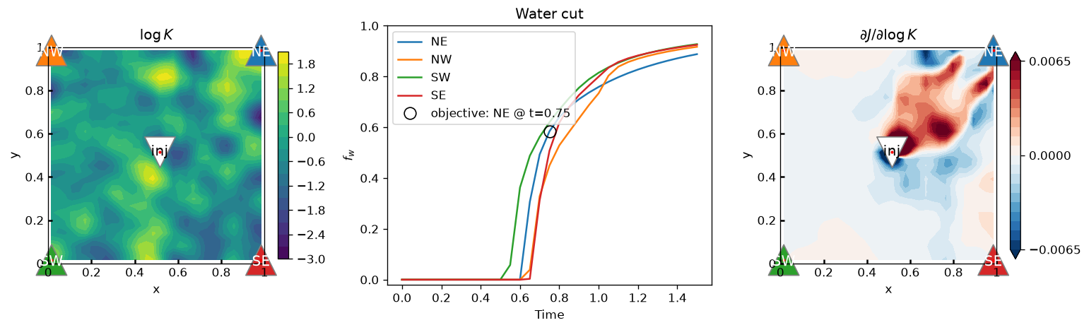
The gradient of the water cut at one producer, at one time, wrt. the field of $\log K$.
A five-spot: one injector at the centre, four producers in the corners, on a
heterogeneous (smoothed, log-normal) permeability. The objective is the water
cut at the NE producer at a time index just after its breakthrough, where it is
rising fastest. TPFA_ResSim.tlm.adjoint returns its gradient with respect to
every cell's $\log K$ (and the initial state) at the cost of about one more
simulation -- here checked against a finite difference in a random direction,
which agrees to about 1e-8.
The water cut at a producer, $ f_w(s) $ in its cell (the fraction of water in
what it produces; at a fixed rate, proportional to its water rate), is a
function of the saturation there alone, so the adjoint is seeded by the single
entry $ ∂J/∂s_k[i_\mathrm{prd}] = f_w'(s) $ -- which tlm.fractional_flow
supplies.
In the figure:
- Left: the $\log K$ field, with the wells.
- Middle: the water cut of each producer over time, the objective marked.
- Right: the gradient. It is positive along the flow path from the injector to the NE producer -- more permeable rock there brings the water sooner -- and negative along the paths to the other producers, and around the NE path: more permeable rock there diverts the water from the NE well, or lets it sweep a wider area (later arrival at the well itself). Outside the drainage area of the injector-NE pair, it vanishes: what happens there has not yet had time to affect the NE well.
The gradient is with respect to the isotropic $\log K$.
model.K holds both components, so the adjoint returns a gradient for
each; as they are set equal here, the gradient of the single field is
their sum, ref tlm.Gradient.logK.
  1"""The gradient of the water cut at one producer, at one time, wrt. the field of $\\log K$.
  2
  3A five-spot: one injector at the centre, four producers in the corners, on a
  4heterogeneous (smoothed, log-normal) permeability. The objective is the water
  5cut at the NE producer at a time index just after its breakthrough, where it is
  6rising fastest. `TPFA_ResSim.tlm.adjoint` returns its gradient with respect to
  7every cell's $\\log K$ (and the initial state) at the cost of about one more
  8simulation -- here checked against a finite difference in a random direction,
  9which agrees to about 1e-8.
 10
 11The water cut at a producer, $ f_w(s) $ in its cell (the fraction of water in
 12what it produces; at a fixed rate, proportional to its water rate), is a
 13function of the saturation there alone, so the adjoint is seeded by the single
 14entry $ ∂J/∂s_k[i_\\mathrm{prd}] = f_w'(s) $ -- which `tlm.fractional_flow`
 15supplies.
 16
 17In the figure:
 18
 19- Left: the $\\log K$ field, with the wells.
 20- Middle: the water cut of each producer over time, the objective marked.
 21- Right: the gradient. It is positive along the flow path from the injector
 22  to the NE producer -- more permeable rock there brings the water sooner --
 23  and negative along the paths to the *other* producers, and around the NE
 24  path: more permeable rock there diverts the water from the NE well, or lets
 25  it sweep a wider area (later arrival at the well itself). Outside the
 26  drainage area of the injector-NE pair, it vanishes: what happens there has
 27  not yet had time to affect the NE well.
 28
 29.. note:: The gradient is with respect to the *isotropic* $\\log K$.
 30
 31    `model.K` holds both components, so the adjoint returns a gradient for
 32    each; as they are set equal here, the gradient of the single field is
 33    their sum, ref `tlm.Gradient.logK`.
 34"""
 35
 36from mpl_tools.place import freshfig
 37import matplotlib.pyplot as plt
 38import numpy as np
 39from scipy.ndimage import uniform_filter as smooth
 40
 41from TPFA_ResSim import ResSim
 42from TPFA_ResSim.plotting import show
 43from TPFA_ResSim.tlm import adjoint, fractional_flow
 44
 45rng = np.random.default_rng(1)  # Reproducibility (the values are regression tested)
 46
 47## Model: a five-spot on heterogeneous permeability
 48model = ResSim(Lx=1, Ly=1, Nx=32, Ny=32, wells=[
 49    dict(xy=[.5, .5], rate=+1  , name="inj"),
 50    dict(xy=[1 , 1 ], rate=-.25, name="NE"),
 51    dict(xy=[0 , 1 ], rate=-.25, name="NW"),
 52    dict(xy=[0 , 0 ], rate=-.25, name="SW"),
 53    dict(xy=[1 , 0 ], rate=-.25, name="SE"),
 54])
 55logK = 3 * smooth(smooth(rng.standard_normal(model.shape)))
 56model.K = np.exp(logK)  # isotropic: broadcast to both components
 57
 58dt, nSteps = .05, 30
 59S0 = np.zeros(model.Nxy)
 60SS, PP = model.sim(dt, nSteps, S0, pbar=False)
 61
 62## The objective: water cut at the NE producer at time `k`
 63producers = model.wells.names[1:]
 64prd = model.xy2ind(*model.wells.xy[1:].T)  # their cells
 65
 66
 67def water_cut(model, SS):
 68    """`(nSteps+1, nPrd)` water cut at each producer, for each stored time."""
 69    return np.array([fractional_flow(model, S)[0][prd] for S in SS])
 70
 71
 72fw = water_cut(model, SS)
 73well, k = 0, 15  # NE, just after breakthrough (fw ≈ .5)
 74J = fw[k, well]
 75
 76## Its gradient, by the adjoint
 77dJ_dSS = np.zeros_like(SS)
 78dJ_dSS[k, prd[well]] = fractional_flow(model, SS[k])[1][prd[well]]  # f_w'(s)
 79grad = adjoint(model, dt, SS, PP, dJ_dSS)
 80G = grad.logK.sum(0)  # isotropic ⇒ sum the components
 81
 82## Check: a finite difference in a random direction of log K
 83direction = rng.standard_normal(model.shape)
 84eps = 1e-5
 85def J_of(logK):  # noqa: E302
 86    m = ResSim(Lx=1, Ly=1, Nx=32, Ny=32, wells=model.wells)
 87    m.K = np.exp(logK)
 88    return water_cut(m, m.sim(dt, nSteps, S0, pbar=False)[0])[k, well]
 89fd = (J_of(logK + eps*direction) - J_of(logK - eps*direction)) / (2*eps)
 90directional = (G * direction).sum()
 91assert abs(fd - directional) < 1e-4 * abs(directional), (fd, directional)
 92
 93## Plot
 94fig, axs = freshfig("Water-cut gradient", ncols=3, figsize=(13, 4),
 95                    gridspec_kw={'width_ratios': (1, 1.2, 1)})
 96
 97ax = axs[0]
 98model.plt_field(ax, logK, title="$\\log K$", cmap="viridis", levels=17,
 99                wells="color", finalize=False)
100
101ax = axs[1]
102tt = dt * np.arange(nSteps + 1)
103for i, name in enumerate(producers):
104    ax.plot(tt, fw[:, i], label=name, c=f"C{i}")
105ax.plot(tt[k], J, "o", c="k", mfc="none", ms=10, zorder=3,
106        label=f"objective: {producers[well]} @ t={tt[k]:.2f}")
107ax.set(title="Water cut", xlabel="Time", ylabel="$f_w$", ylim=(-.02, 1))
108ax.legend(loc="upper left")
109
110ax = axs[2]
111# The few cells next to the wells dominate; clip the color scale (the cmap's
112# `over`/`under` make `plt_field` extend the colorbar, rather than leave blanks).
113m = np.percentile(abs(G), 98)
114cmap = plt.get_cmap("RdBu_r")
115cmap = cmap.with_extremes(over=cmap(1.0), under=cmap(0.0))
116model.plt_field(ax, G, title="$∂J/∂\\log K$", cmap=cmap,
117                levels=np.linspace(-m, m, 21), cticks=[-m, 0, m],
118                wells="color", finalize=False)
119
120fig.tight_layout()
121
122# Regression values, checked by `tests/test_examples.py`.
123__digest__ = dict(water_cut   = fw,
124                  gradient    = G,
125                  directional = [directional, fd])
126
127if __name__ == "__main__":
128    show()